pacman::p_load(sf, tidyverse, tmap, jsonlite, rvest, onemapsgapi, olsrr, corrplot, ggpubr, spdep, GWmodel, gtsummary, ggthemes, zoo, SpatialML, tmap, rsample, Metrics, matrixStats, kableExtra)Take Home Exercise 3
1 Setting The Scene
Housing is an essential component of household wealth worldwide. Buying a housing has always been a major investment for most people. The price of housing is affected by many factors. Some of them are global in nature such as the general economy of a country or inflation rate. Others can be more specific to the properties themselves. These factors can be further divided to structural and locational factors. Structural factors are variables related to the property themselves such as the size, fitting, and tenure of the property. Locational factors are variables related to the neighbourhood of the properties such as proximity to childcare centre, public transport service and shopping centre.
Conventional, housing resale prices predictive models were built by using Ordinary Least Square (OLS) method. However, this method failed to take into consideration that spatial autocorrelation and spatial heterogeneity exist in geographic data sets such as housing transactions. With the existence of spatial autocorrelation, the OLS estimation of predictive housing resale pricing models could lead to biased, inconsistent, or inefficient results (Anselin 1998). In view of this limitation, Geographical Weighted Models were introduced for calibrating predictive model for housing resale prices.
2 The Task
In this take-home exercise, you are tasked to predict HDB resale prices at the sub-market level (i.e. HDB 3-room, HDB 4-room and HDB 5-room) for the month of January and February 2023 in Singapore. The predictive models must be built by using by using conventional OLS method and GWR methods. You are also required to compare the performance of the conventional OLS method versus the geographical weighted methods.
3 Importing Required R Packages
The following packages are used in this assignment
Building Ordinary Least Square model and performing diagnostics tests
Calibrating geographical weighted family of models
Multivariate data visualisation and analysis
Random Forest model generation
Converting JSON objects to R data types
Spatial data handling
- sf
Attribute data handling
- tidyverse, especially readr, ggplot2 and dplyr
Choropleth mapping
- tmap
Handling spatial autocorrelation calculations
For API queries calls for Singapore specific data
Summarising model statistics
4 The Data
Structural and Locational factors will be extracted:
Structural factors
Area of the unit
Floor level
Remaining lease
Age of the unit
Locational factors
Proxomity to CBD
Proximity to eldercare
Proximity to hawker centres
Proximity to MRT
Proximity to park
Proximity to good primary school
Proximity to shopping mall
Proximity to supermarket
Number of kindergartens within 350m
Number of childcare centres within 350m
Number of bus stop within 350m
Number of primary schools within 1km
The following table describes the data sources used in this assignment.
Show Code
datasets <- data.frame(
Type=c("Aspatial",
"Geospatial",
"Geospatial - Extracted",
"Geospatial",
"Geospatial",
"Geospatial",
"Geospatial",
"Geospatial - Extracted",
"Geospatial - Extracted",
"Geospatial - Extracted",
"Geospatial - Extracted",
"Geospatial",
"Geospatial",
"Geospatial"
),
Name=c("Resale Flat Prices",
"Master Plan 2019 Subzone Boundary (Web)",
"Central Business District Coordinates",
"Eldercare Services",
"Hawker Centres",
"MRT Stations",
"Parks",
"Good Primary Schools",
"Shopping Mall",
"Supermarkets",
"Kindergartens",
"Childcare Services",
"Bus Stops",
"Primary Schools"),
Format=c(".csv",
".shp",
".shp",
".shp",
".geojson",
".shp",
".kml",
".shp",
".geojson",
".geojson",
".shp",
".geojson",
".shp",
".xlsx"
),
Source=c("[data.gov.sg](https://data.gov.sg/dataset/resale-flat-prices)",
"[In-Class Ex 9](https://data.gov.sg/dataset/master-plan-2019-subzone-boundary-no-sea)",
"[latlong.net](https://www.latlong.net/place/downtown-core-singapore-20616.html)",
"[data.gov.sg](https://data.gov.sg/dataset/eldercare-services)",
"[data.gov.sg](https://data.gov.sg/dataset/hawker-centres)",
"[Datamall](https://datamall.lta.gov.sg/content/dam/datamall/datasets/Geospatial/TrainStationExit.zip)",
"[data.gov.sg](https://data.gov.sg/dataset/parks)",
"[salary.sg](https://www.salary.sg/2022/best-primary-schools-2022-by-popularity/)",
"[Mall SVY21 Coordinates Web Scaper](https://github.com/ValaryLim/Mall-Coordinates-Web-Scraper)",
"[data.gov.sg](https://data.gov.sg/dataset/supermarkets)",
"[OneMap API](https://www.onemap.gov.sg/docs/)",
"[Hands-on Ex 3](https://annatrw-is415.netlify.app/hands-on_ex/hands-on_ex03/hands-on_ex03)",
"[Datamall](https://datamall.lta.gov.sg/content/dam/datamall/datasets/Geospatial/BusStopLocation.zip)",
"[data.gov.sg](https://data.gov.sg/dataset/school-directory-and-information)"
)
)
# with reference to this guide on kableExtra:
# https://cran.r-project.org/web/packages/kableExtra/vignettes/awesome_table_in_html.html
# kable_material is the name of the kable theme
# 'hover' for to highlight row when hovering, 'scale_down' to adjust table to fit page width
library(knitr)
kable(datasets, caption="Datasets Used") %>%
kable_material("hover", latex_options="scale_down")| Type | Name | Format | Source |
|---|---|---|---|
| Aspatial | Resale Flat Prices | .csv | [data.gov.sg](https://data.gov.sg/dataset/resale-flat-prices) |
| Geospatial | Master Plan 2019 Subzone Boundary (Web) | .shp | [In-Class Ex 9](https://data.gov.sg/dataset/master-plan-2019-subzone-boundary-no-sea) |
| Geospatial - Extracted | Central Business District Coordinates | .shp | [latlong.net](https://www.latlong.net/place/downtown-core-singapore-20616.html) |
| Geospatial | Eldercare Services | .shp | [data.gov.sg](https://data.gov.sg/dataset/eldercare-services) |
| Geospatial | Hawker Centres | .geojson | [data.gov.sg](https://data.gov.sg/dataset/hawker-centres) |
| Geospatial | MRT Stations | .shp | [Datamall](https://datamall.lta.gov.sg/content/dam/datamall/datasets/Geospatial/TrainStationExit.zip) |
| Geospatial | Parks | .kml | [data.gov.sg](https://data.gov.sg/dataset/parks) |
| Geospatial - Extracted | Good Primary Schools | .shp | [salary.sg](https://www.salary.sg/2022/best-primary-schools-2022-by-popularity/) |
| Geospatial - Extracted | Shopping Mall | .geojson | [Mall SVY21 Coordinates Web Scaper](https://github.com/ValaryLim/Mall-Coordinates-Web-Scraper) |
| Geospatial - Extracted | Supermarkets | .geojson | [data.gov.sg](https://data.gov.sg/dataset/supermarkets) |
| Geospatial - Extracted | Kindergartens | .shp | [OneMap API](https://www.onemap.gov.sg/docs/) |
| Geospatial | Childcare Services | .geojson | [Hands-on Ex 3](https://annatrw-is415.netlify.app/hands-on_ex/hands-on_ex03/hands-on_ex03) |
| Geospatial | Bus Stops | .shp | [Datamall](https://datamall.lta.gov.sg/content/dam/datamall/datasets/Geospatial/BusStopLocation.zip) |
| Geospatial | Primary Schools | .xlsx | [data.gov.sg](https://data.gov.sg/dataset/school-directory-and-information) |
5 Structural Factors
5.1 Import HDB Resale Prices Data
Using read_csv(), import the HDB resale price data.
resale_all <- read_csv("data/aspatial/resale-flat-prices-based-on-registration-date-from-jan-2017-onwards.csv")This is how the resale data looks like.
glimpse(resale_all)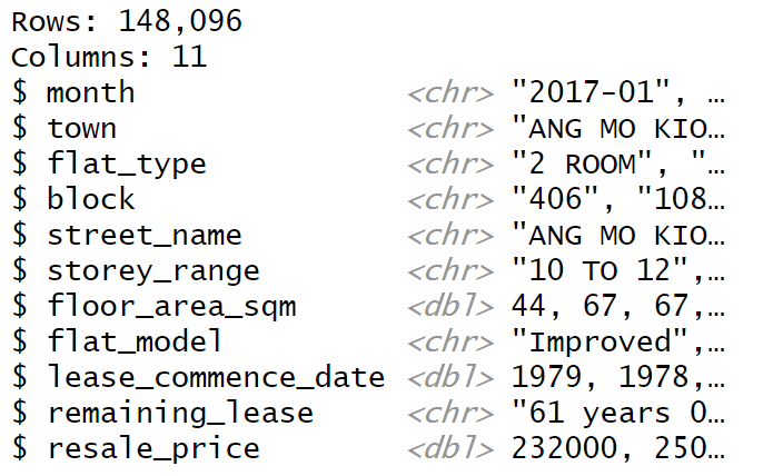
Filter out 2021 and 2022 data as per assignment requirement using grepl().
resale2122 <- filter(resale_all, grepl('2021', month)|grepl('2022', month))Filter out 2023 data for testing.
resale23_test <- filter(resale_all, grepl('2023', month))For the purposes of this assignment, we will be focusing on 5 Room HDB resale flat prices.
unique(resale2122$flat_type)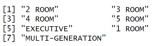
resale2122_5r <- filter(resale2122, flat_type == '5 ROOM')resale23_test <- filter(resale23_test, flat_type == '5 ROOM')5.2 Geocode Resale Data
Referencing senior’s work, this geocoding function using OneMap API will retrieve the latitude and longitude for resale data.
library(httr)
geocode_function <- function(block, street_name) {
base_url <- "https://developers.onemap.sg/commonapi/search"
address <- paste(block, street_name, sep = " ")
query <- list("searchVal" = address,
"returnGeom" = "Y",
"getAddrDetails" = "N",
"pageNum" = "1")
res <- GET(base_url, query = query)
restext<-content(res, as="text")
output <- fromJSON(restext) %>%
as.data.frame %>%
select(results.LATITUDE, results.LONGITUDE)
return(output)
}resale2122_5r$street_name <- gsub("ST\\.", "SAINT", resale2122_5r$street_name)Execute the geocoding function
resale2122_5r$LATITUDE <- 0
resale2122_5r$LONGITUDE <- 0
for (i in 1:nrow(resale2122_5r)){
temp_output <- geocode_function(resale2122_5r[i, 4], resale2122_5r[i, 5])
resale2122_5r$LATITUDE[i] <- temp_output$results.LATITUDE
resale2122_5r$LONGITUDE[i] <- temp_output$results.LONGITUDE
}We check if there are null values in the coordinate columns, in which there are none.
sum(is.na(resale2122_5r$LATITUDE))sum(is.na(resale2122_5r$LONGITUDE))resale23_test$street_name <- gsub("ST\\.", "SAINT", resale23_test$street_name)Execute the geocoding function
resale23_test$LATITUDE <- 0
resale23_test$LONGITUDE <- 0
for (i in 1:nrow(resale23_test)){
temp_output <- geocode_function(resale23_test[i, 4], resale23_test[i, 5])
resale23_test$LATITUDE[i] <- temp_output$results.LATITUDE
resale23_test$LONGITUDE[i] <- temp_output$results.LONGITUDE
}sum(is.na(resale23_test$LATITUDE))sum(is.na(resale23_test$LONGITUDE))5.3 Remaining Lease
Referencing senior’s work, the remaining lease in years is retrieved by converting years and months into years.
str_list <- str_split(resale2122_5r$remaining_lease, " ")
for (i in 1:length(str_list)) {
if (length(unlist(str_list[i])) > 2) {
year <- as.numeric(unlist(str_list[i])[1])
month <- as.numeric(unlist(str_list[i])[3])
resale2122_5r$remaining_lease[i] <- year + round(month/12, 2)
}
else {
year <- as.numeric(unlist(str_list[i])[1])
resale2122_5r$remaining_lease[i] <- year
}
}str_list <- str_split(resale23_test$remaining_lease, " ")
for (i in 1:length(str_list)) {
if (length(unlist(str_list[i])) > 2) {
year <- as.numeric(unlist(str_list[i])[1])
month <- as.numeric(unlist(str_list[i])[3])
resale23_test$remaining_lease[i] <- year + round(month/12, 2)
}
else {
year <- as.numeric(unlist(str_list[i])[1])
resale23_test$remaining_lease[i] <- year
}
}5.4 Floor Level
Referencing senior’s work, the floor level is retrieved by first sorting the storeys in ascending order, then assigning a numerical value to each category.
storeys <- sort(unique(resale2122_5r$storey_range))storey_order <- 1:length(storeys)
storey_range_order <- data.frame(storeys, storey_order)resale2122_5r <- left_join(resale2122_5r, storey_range_order, by= c("storey_range" = "storeys"))storeys <- sort(unique(resale23_test$storey_range))storey_order <- 1:length(storeys)
storey_range_order <- data.frame(storeys, storey_order)resale23_test <- left_join(resale23_test, storey_range_order, by= c("storey_range" = "storeys"))5.5 Age of Unit
Convert the date field to a date data type, which assumes the first day of the month since date is in yyyy/mm format; referencing sources online.
date <- as.Date(as.yearmon(resale2122_5r$month))
resale2122_5r$start <- as.numeric(format(date,'%Y'))Age of unit calculation will only consider the year when the flat was sold.
resale2122_5r$UNIT_AGE <- resale2122_5r$start - resale2122_5r$lease_commence_datedate <- as.Date(as.yearmon(resale23_test$month))
resale23_test$start <- as.numeric(format(date,'%Y'))
resale23_test$UNIT_AGE <- resale23_test$start - resale23_test$lease_commence_date5.6 Convert Resale Data To sf Object
Convert the dataframe into an sf object with geometry field attached, referencing here.
resale2122_5r_sf <- st_as_sf(resale2122_5r,
coords = c("LONGITUDE",
"LATITUDE"),
# the geographical features are in longitude & latitude, in decimals
# as such, WGS84 is the most appropriate coordinates system
crs=4326) %>%
#afterwards, we transform it to SVY21, our desired CRS
st_transform(crs = 3414)resale23_test_sf <- st_as_sf(resale23_test,
coords = c("LONGITUDE",
"LATITUDE"),
# the geographical features are in longitude & latitude, in decimals
# as such, WGS84 is the most appropriate coordinates system
crs=4326) %>%
#afterwards, we transform it to SVY21, our desired CRS
st_transform(crs = 3414)6 Locational Factors
As mentioned, the following locational factors will be used for predictive modelling of HDB resale prices.
- Proximity to CBD
- Proximity to eldercare services
- Proximity to hawker centres
- Proximity to MRT stations
- Proximity to parks
- Proximity to good primary schools
- proximity to shopping malls
- proximity to supermarkets
- Number of kindergarten within 350m
- Number of child care services within 350m
- Number of bus stops within 350m
- Number of primary schools within 1km
6.1 Factors With Geographic Coordinates
6.1.1 Self-sourced and referenced
6.1.1.1 Kindergartens
Using OneMap API retrieval methods, my personal token was pre-loaded into the token variable and used to call the OneMap API to retrieve location of kindergartens in Singapore as an sf object.
search_themes(token, "kindergarten")
get_theme_status(token, "kindergartens")
themetibble <- get_theme(token, "kindergartens")
kindergarten_sf <- st_as_sf(themetibble, coords=c("Lng", "Lat"), crs=4326)6.1.1.2 Shopping Malls
With reference to a previously done project to scrape the locations of shopping malls in Singapore, read in the csv and convert it to an sf object with appropriate projection system.
mall_csv <- read_csv("data/geospatial/mall_coordinates_updated.csv")glimpse(mall_csv)malls_sf <- st_as_sf(mall_csv,
coords = c("longitude",
"latitude"),
crs=4326) %>%
st_transform(crs = 3414)6.1.2 Geojson Sources
Import the geojson files.
elder_sf <- st_read(dsn = "data/geospatial/ElderCare", layer="ELDERCARE")
mrt_sf <- st_read(dsn = "data/geospatial/TrainStationExit", layer="Train_Station_Exit_Layer")
bus_sf <- st_read(dsn = "data/geospatial/BusStop_Feb2023", layer="BusStop")
hawker_sf <- st_read("data/geospatial/hawker-centres-geojson.geojson")
parks_sf <- st_read("data/geospatial/parks.kml")
supermkt_sf <- st_read("data/geospatial/supermarkets-geojson.geojson")
childcare_sf <- st_read("data/geospatial/child-care-services-geojson.geojson")
mpsz_sf <- st_read(dsn="data/geospatial/MPSZ2019", layer = "MPSZ-2019") 6.1.2.1 CRS
Check the CRS projection for the layers.
st_crs(elder_sf)
st_crs(mrt_sf)
st_crs(bus_sf)
st_crs(hawker_sf)
st_crs(parks_sf)
st_crs(supermkt_sf)
st_crs(childcare_sf)
st_crs(mpsz_sf)
st_crs(kindergarten_sf)
st_crs(malls_sf)They are projected wrongly - using EPSG 9001 - when it should be projected to EPSG 4326 instead.
Set correct CRS except for malls_sf which is already EPSG 3414 done in previous section when transforming to sf object.
mpsz_sf <- st_set_crs(mpsz_sf, 3414)
elder_sf <- st_set_crs(elder_sf, 3414)
mrt_sf <- st_set_crs(mrt_sf, 3414)
bus_sf <- st_set_crs(bus_sf, 3414)
hawker_sf <- hawker_sf %>%
st_transform(crs = 3414)
parks_sf <- parks_sf %>%
st_transform(crs = 3414)
supermkt_sf <- supermkt_sf %>%
st_transform(crs = 3414)
childcare_sf <- childcare_sf %>%
st_transform(crs = 3414)
kindergarten_sf <- kindergarten_sf %>%
st_transform(crs = 3414)Verify that there are no invalid geometries:
length(which(st_is_valid(mpsz_sf) == FALSE))
length(which(st_is_valid(elder_sf) == FALSE))
length(which(st_is_valid(mrt_sf) == FALSE))
length(which(st_is_valid(bus_sf) == FALSE))
length(which(st_is_valid(hawker_sf) == FALSE))
length(which(st_is_valid(supermkt_sf) == FALSE))
length(which(st_is_valid(parks_sf) == FALSE))
length(which(st_is_valid(childcare_sf) == FALSE))
length(which(st_is_valid(kindergarten_sf) == FALSE))
length(which(st_is_valid(malls_sf) == FALSE))There are invalid geometries for mpsz_sf; which can be rectified with st_make_valid().
mpsz_sf <- sf::st_make_valid(mpsz_sf)
length(which(st_is_valid(mpsz_sf) == FALSE))6.1.3 Calculate Proximity
Using a proximity function from senior’s work, st_distance is used to compute a distance matrix which will retrieve the minimum distance from origin to destination.
get_prox <- function(origin_df, dest_df, col_name){
# creates a matrix of distances
dist_matrix <- st_distance(origin_df, dest_df)
# find the nearest location_factor and create new data frame
near <- origin_df %>%
mutate(PROX = apply(dist_matrix, 1, function(x) min(x)) / 1000)
# rename column name according to input parameter
names(near)[names(near) == 'PROX'] <- col_name
# Return df
return(near)
}resale2122_5r_sf <- get_prox(resale2122_5r_sf, elder_sf, "PROX_ELDERCARE")
resale2122_5r_sf <- get_prox(resale2122_5r_sf, mrt_sf, "PROX_MRT")
resale2122_5r_sf <- get_prox(resale2122_5r_sf, hawker_sf, "PROX_HAWKER")
resale2122_5r_sf <- get_prox(resale2122_5r_sf, parks_sf, "PROX_PARK")
resale2122_5r_sf <- get_prox(resale2122_5r_sf, supermkt_sf, "PROX_SUPERMARKET")
resale2122_5r_sf <- get_prox(resale2122_5r_sf, malls_sf, "PROX_MALL")resale23_test_sf <- get_prox(resale23_test_sf, elder_sf, "PROX_ELDERCARE")
resale23_test_sf <- get_prox(resale23_test_sf, mrt_sf, "PROX_MRT")
resale23_test_sf <- get_prox(resale23_test_sf, hawker_sf, "PROX_HAWKER")
resale23_test_sf <- get_prox(resale23_test_sf, parks_sf, "PROX_PARK")
resale23_test_sf <- get_prox(resale23_test_sf, supermkt_sf, "PROX_SUPERMARKET")
resale23_test_sf <- get_prox(resale23_test_sf, malls_sf, "PROX_MALL")6.2 Calculate Number of Amenities
Using a function to get the number of amenities within a certain distance from senior’s work, the get within function counts the number of amenities within the threshold distance.
get_within <- function(origin_df, dest_df, threshold_dist, col_name){
# creates a matrix of distances
dist_matrix <- st_distance(origin_df, dest_df)
# count the number of location_factors within threshold_dist and create new data frame
wdist <- origin_df %>%
mutate(WITHIN_DT = apply(dist_matrix, 1, function(x) sum(x <= threshold_dist)))
# rename column name according to input parameter
names(wdist)[names(wdist) == 'WITHIN_DT'] <- col_name
# Return df
return(wdist)
}6.2.0.1 Number of Kindergartens Within 350m
resale2122_5r_sf <- get_within(resale2122_5r_sf, kindergarten_sf, 350, "WITHIN_350M_KINDERGARTEN")6.2.0.2 Number of Childcare Centres Within 350m
resale2122_5r_sf <- get_within(resale2122_5r_sf, childcare_sf, 350, "WITHIN_350M_CHILDCARE")6.2.0.3 Number of Bus Stops Within 350m
resale2122_5r_sf <- get_within(resale2122_5r_sf, bus_sf, 350, "WITHIN_350M_BUS")6.2.0.4 Number of Kindergartens Within 350m
resale23_test_sf <- get_within(resale23_test_sf, kindergarten_sf, 350, "WITHIN_350M_KINDERGARTEN")6.2.0.5 Number of Childcare Centres Within 350m
resale23_test_sf <- get_within(resale23_test_sf, childcare_sf, 350, "WITHIN_350M_CHILDCARE")6.2.0.6 Number of Bus Stops Within 350m
resale23_test_sf <- get_within(resale23_test_sf, bus_sf, 350, "WITHIN_350M_BUS")6.3 Factors Without Geographic Coordinates
6.3.1 CBD
Get the coordinates of Singapore’s Central Business District in Downtown Core using latlong.net: 1.287953, 103.851784
name <- c('CBD')
latitude= c(1.287953)
longitude= c(103.851784)
cbd <- data.frame(name, latitude, longitude)cbd_sf <- st_as_sf(cbd, coords = c("longitude", "latitude"), crs = 4326) %>%
st_transform(crs = 3414)st_crs(cbd_sf)Upon checking, the CBD data is in the correct CRS.
6.3.1.1 Get Proximity To CBD
This is done by calling the earlier defined get_prox function.
resale2122_5r_sf <- get_prox(resale2122_5r_sf, cbd_sf, "PROX_CBD") resale23_test_sf <- get_prox(resale23_test_sf, cbd_sf, "PROX_CBD") 6.3.2 Primary Schools
Read the csv of schools and filter out the primary schools for study.
pri_sch <- read_csv("data/geospatial/general-information-of-schools.csv")pri_sch <- pri_sch %>%
filter(mainlevel_code == "PRIMARY") %>%
select(school_name, address, postal_code, mainlevel_code)glimpse(pri_sch)6.3.2.1 Geocode
Referencing this link, define a get_coords() function that utilises the OneMap API, feeding the postal codes through it to get latitude and longitude.
get_coords <- function(add_list){
# Create a data frame to store all retrieved coordinates
postal_coords <- data.frame()
for (i in add_list){
#print(i)
r <- GET('https://developers.onemap.sg/commonapi/search?',
query=list(searchVal=i,
returnGeom='Y',
getAddrDetails='Y'))
data <- fromJSON(rawToChar(r$content))
found <- data$found
res <- data$results
# Create a new data frame for each address
new_row <- data.frame()
# If single result, append
if (found == 1){
postal <- res$POSTAL
lat <- res$LATITUDE
lng <- res$LONGITUDE
new_row <- data.frame(address= i, postal = postal, latitude = lat, longitude = lng)
}
# If multiple results, drop NIL and append top 1
else if (found > 1){
# Remove those with NIL as postal
res_sub <- res[res$POSTAL != "NIL", ]
# Set as NA first if no Postal
if (nrow(res_sub) == 0) {
new_row <- data.frame(address= i, postal = NA, latitude = NA, longitude = NA)
}
else{
top1 <- head(res_sub, n = 1)
postal <- top1$POSTAL
lat <- top1$LATITUDE
lng <- top1$LONGITUDE
new_row <- data.frame(address= i, postal = postal, latitude = lat, longitude = lng)
}
}
else {
new_row <- data.frame(address= i, postal = NA, latitude = NA, longitude = NA)
}
# Add the row
postal_coords <- rbind(postal_coords, new_row)
}
return(postal_coords)
}We extract the unique postal codes and feed them through the get_coords function.
prisch_postal <- sort(unique(pri_sch$postal_code))prisch_coords <- get_coords(prisch_postal)This code checks for any null values in the retrieved coordinates data.
prisch_coords[(is.na(prisch_coords$postal) | is.na(prisch_coords$latitude) | is.na(prisch_coords$longitude)), ]glimpse(prisch_coords)We can safely combine the retrieved coordinates with the original primary schools csv data.
prisch_coords = prisch_coords[c("postal","latitude", "longitude")]
pri_sch <- left_join(pri_sch, prisch_coords, by = c('postal_code' = 'postal'))Lastly, we convert to it to an sf object with the correct projection.
prisch_sf <- st_as_sf(pri_sch,
coords = c("longitude",
"latitude"),
crs=4326) %>%
st_transform(crs = 3414)6.3.2.2 Number of Primary Schools Within 1km
Run the primary schools data through the get_within function to get the number of primary schools within 1km.
resale2122_5r_sf <- get_within(resale2122_5r_sf, prisch_sf, 1000, "WITHIN_1KM_PRISCH")resale23_test_sf <- get_within(resale23_test_sf, prisch_sf, 1000, "WITHIN_1KM_PRISCH")6.4 Good Primary Schools
With reference to salary.sg, we can extract the top 10 primary schools in 2022. Using the method employed by senior, the following web crawling method is used to search for the html element - which is a list item - on the web page to retrieve the top 10 primary schools.
url <- "https://www.salary.sg/2022/best-primary-schools-2022-by-popularity/"
good_pri <- data.frame()
schools <- read_html(url) %>%
html_nodes(xpath = paste('//*[@id="post-33132"]/div[3]/div/div/ol/li') ) %>%
html_text()
for (i in (schools)){
sch_name <- toupper(gsub(" – .*","",i))
sch_name <- gsub("\\(PRIMARY SECTION)","",sch_name)
sch_name <- trimws(sch_name)
new_row <- data.frame(pri_sch_name=sch_name)
# Add the row
good_pri <- rbind(good_pri, new_row)
}
top_good_pri <- head(good_pri, 10)top_good_pri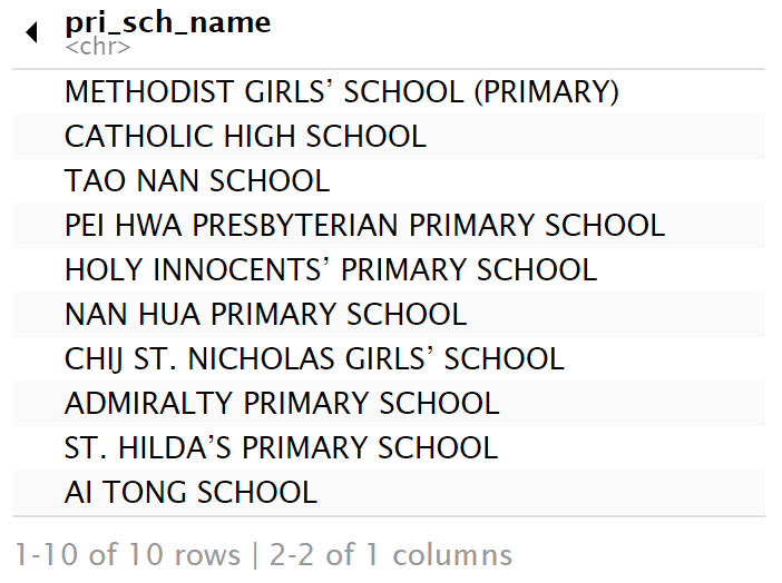
Check which top schools are not in prisch_sf.
top_good_pri$pri_sch_name[!top_good_pri$pri_sch_name %in% prisch_sf$school_name]Get the coordinates list of good primary schools and check for null values, upon which we see that St Hilda’s primary school does not exist in the prisch_sf data.
good_pri_list <- unique(top_good_pri$pri_sch_name)
good_pri_listgoodprisch_coords <- get_coords(good_pri_list)
goodprisch_coordsgoodprisch_coords[(is.na(goodprisch_coords$postal) | is.na(goodprisch_coords$latitude) | is.na(goodprisch_coords$longitude)), ]To rectify this, change the apostrophe symbol for the school title “ST HILDA’S PRIMARY SCHOOL”.
top_good_pri$pri_sch_name[top_good_pri$pri_sch_name == "ST. HILDA’S PRIMARY SCHOOL"] <- "ST. HILDA'S PRIMARY SCHOOL"Here, we check once again for null values in the new coordinates list.
good_pri_list <- unique(top_good_pri$pri_sch_name)
good_pri_listgoodprisch_coords <- get_coords(good_pri_list)
goodprisch_coordsgoodprisch_coords[(is.na(goodprisch_coords$postal) | is.na(goodprisch_coords$latitude) | is.na(goodprisch_coords$longitude)), ]Finally, convert the layer into an sf object with the correct projection.
good_pri_sf <- st_as_sf(goodprisch_coords,
coords = c("longitude",
"latitude"),
crs=4326) %>%
st_transform(crs = 3414)resale2122_5r_sf <- get_prox(resale2122_5r_sf, good_pri_sf, "PROX_GOOD_PRISCH")resale23_test_sf <- get_prox(resale23_test_sf, good_pri_sf, "PROX_GOOD_PRISCH")6.5 Other Data Processing
For the last steps of data processing, we retain necessary columns by dropping unnecessary one using subset() as well as convert the remaining lease field from a string data type to numeric.
resale2122_5r_sf <- subset(resale2122_5r_sf, select = -c(month, town, flat_type, storey_range, block, street_name, flat_model, lease_commence_date, start)) %>% select(resale_price, everything())resale2122_5r_sf$remaining_lease <- as.numeric(resale2122_5r_sf$remaining_lease)glimpse(resale2122_5r_sf)resale23_test_sf <- subset(resale23_test_sf, select = -c(month, town, flat_type, storey_range, block, street_name, flat_model, lease_commence_date, start)) %>% select(resale_price, everything())resale23_test_sf$remaining_lease <- as.numeric(resale23_test_sf$remaining_lease)6.6 Write Data To rds File
Save the train and test data that are sf objects into an rds file to reduce the computation and render time, as well as for easy access.
train <- write_rds(resale2122_5r_sf, "data/rds/factors.rds")test <- write_rds(resale23_test_sf, "data/rds/factors_test.rds")7 EDA
Since we are building a predictive model, load the train and test data separately.
train <- read_rds("data/rds/factors.rds")
test <- read_rds("data/rds/factors_test.rds")Our training data has 14,519 rows and 18 columns as shown below.
glimpse(train)Rows: 14,519
Columns: 18
$ resale_price <dbl> 483000, 590000, 629000, 670000, 680000, 76000…
$ floor_area_sqm <dbl> 118, 123, 118, 128, 133, 133, 110, 110, 110, …
$ remaining_lease <dbl> 59.08, 55.58, 58.67, 74.25, 71.25, 74.50, 84.…
$ storey_order <int> 1, 5, 6, 3, 1, 5, 8, 5, 6, 6, 5, 5, 8, 1, 2, …
$ UNIT_AGE <dbl> 40, 44, 41, 25, 28, 25, 15, 19, 15, 10, 10, 1…
$ geometry <POINT [m]> POINT (30820.82 39547.58), POINT (29412…
$ PROX_ELDERCARE <dbl> 1.0646617, 0.1908834, 0.7891907, 0.1476040, 0…
$ PROX_MRT <dbl> 1.0808607, 0.5243923, 0.4159309, 0.2427019, 0…
$ PROX_HAWKER <dbl> 0.4828156, 0.3317637, 0.3792242, 0.5884497, 0…
$ PROX_PARK <dbl> 0.7359373, 0.5808933, 0.3087999, 0.2838337, 0…
$ PROX_SUPERMARKET <dbl> 0.41991387, 0.24554343, 0.31805791, 0.3135757…
$ PROX_MALL <dbl> 1.2132871, 0.4416229, 0.5494572, 1.5369839, 0…
$ WITHIN_350M_KINDERGARTEN <int> 1, 1, 1, 1, 1, 1, 1, 0, 1, 1, 1, 1, 1, 0, 0, …
$ WITHIN_350M_CHILDCARE <int> 2, 5, 3, 3, 2, 3, 5, 2, 5, 4, 5, 4, 4, 2, 2, …
$ WITHIN_350M_BUS <int> 2, 8, 6, 11, 6, 8, 4, 9, 5, 9, 7, 9, 9, 7, 6,…
$ PROX_CBD <dbl> 9.537543, 8.663223, 9.449166, 9.211988, 8.935…
$ WITHIN_1KM_PRISCH <int> 1, 3, 2, 3, 3, 3, 4, 2, 2, 2, 2, 2, 2, 3, 2, …
$ PROX_GOOD_PRISCH <dbl> 2.6201989, 1.2626796, 1.8786592, 0.4463958, 1…View the summary of the training data to get a quick sense of the data spread and values contained in it.
summary(train) resale_price floor_area_sqm remaining_lease storey_order
Min. : 350000 Min. : 99.0 Min. :49.08 Min. : 1.000
1st Qu.: 528000 1st Qu.:112.0 1st Qu.:69.92 1st Qu.: 2.000
Median : 595000 Median :115.0 Median :77.83 Median : 3.000
Mean : 627297 Mean :117.4 Mean :77.61 Mean : 3.514
3rd Qu.: 690000 3rd Qu.:122.0 3rd Qu.:89.08 3rd Qu.: 5.000
Max. :1418000 Max. :167.0 Max. :96.75 Max. :17.000
UNIT_AGE geometry PROX_ELDERCARE PROX_MRT
Min. : 2.00 POINT :14519 Min. :0.0000 Min. :0.02293
1st Qu.:10.00 epsg:3414 : 0 1st Qu.:0.3561 1st Qu.:0.25435
Median :21.00 +proj=tmer...: 0 Median :0.6375 Median :0.43919
Mean :21.45 Mean :0.8264 Mean :0.53943
3rd Qu.:29.00 3rd Qu.:1.1393 3rd Qu.:0.72288
Max. :50.00 Max. :8.2660 Max. :2.12909
PROX_HAWKER PROX_PARK PROX_SUPERMARKET PROX_MALL
Min. :0.04949 Min. :0.06004 Min. :0.0000007 Min. :0.0000
1st Qu.:0.44137 1st Qu.:0.48334 1st Qu.:0.1808138 1st Qu.:0.3669
Median :0.76583 Median :0.71014 Median :0.2784712 Median :0.5474
Mean :0.88310 Mean :0.79447 Mean :0.2984345 Mean :0.6301
3rd Qu.:1.17913 3rd Qu.:1.01433 3rd Qu.:0.3934945 3rd Qu.:0.8079
Max. :6.63383 Max. :6.00302 Max. :1.6713100 Max. :4.0092
WITHIN_350M_KINDERGARTEN WITHIN_350M_CHILDCARE WITHIN_350M_BUS
Min. :0.000 Min. : 0.000 Min. : 0.000
1st Qu.:0.000 1st Qu.: 3.000 1st Qu.: 6.000
Median :1.000 Median : 4.000 Median : 8.000
Mean :1.075 Mean : 3.952 Mean : 8.141
3rd Qu.:1.000 3rd Qu.: 5.000 3rd Qu.:10.000
Max. :8.000 Max. :20.000 Max. :19.000
PROX_CBD WITHIN_1KM_PRISCH PROX_GOOD_PRISCH
Min. : 1.611 Min. :0.000 Min. : 0.07958
1st Qu.:10.637 1st Qu.:2.000 1st Qu.: 2.05408
Median :13.509 Median :3.000 Median : 3.17117
Mean :12.704 Mean :3.419 Mean : 3.37962
3rd Qu.:15.250 3rd Qu.:4.000 3rd Qu.: 4.60464
Max. :23.277 Max. :9.000 Max. :13.01618 7.1 EDA with Statistical Graphs
summary(train$resale_price) Min. 1st Qu. Median Mean 3rd Qu. Max.
350000 528000 595000 627297 690000 1418000 ggplot(data=train, aes(x=`resale_price`)) +
geom_histogram(bins=20, color="black", fill="light blue")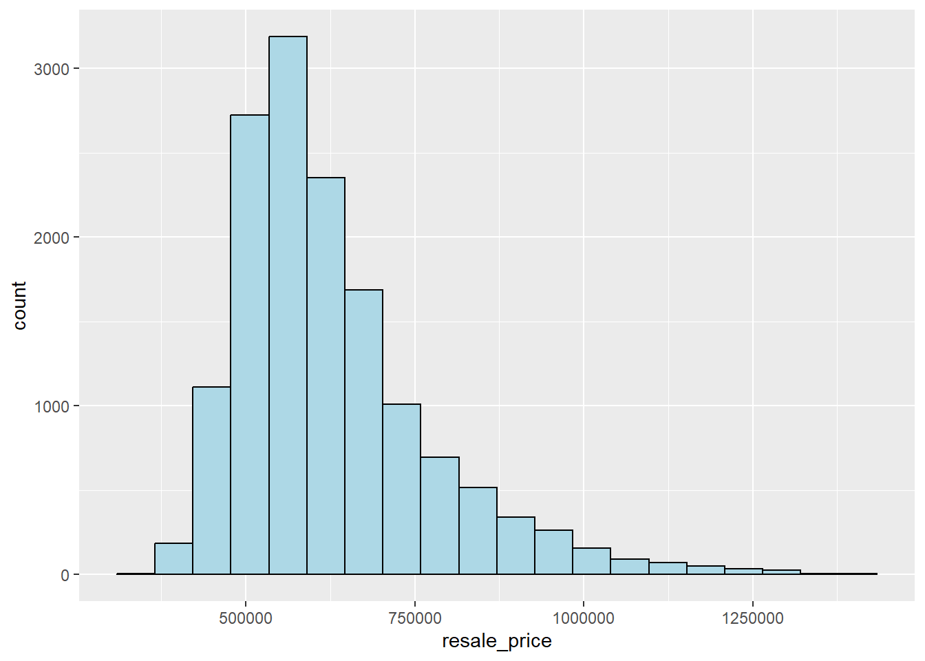
From the histogram, We can observe a right skewed distribution of HDB resale prices in 2021 to 2022.
To visualise the shape of independent variables, use a multiple histogram plot below.
FLOOR_AREA_SQM <- ggplot(data=train, aes(x= `floor_area_sqm`)) +
geom_histogram(bins=20, color="black", fill="light blue")
LEASE_YRS <- ggplot(data=train, aes(x= `remaining_lease`)) +
geom_histogram(bins=20, color="black", fill="light blue")
STOREY_ORDER <- ggplot(data=train, aes(x= `storey_order`)) +
geom_histogram(bins=20, color="black", fill="light blue")
UNIT_AGE <- ggplot(data=train, aes(x= `UNIT_AGE`)) +
geom_histogram(bins=20, color="black", fill="light blue")
PROX_ELDERCARE <- ggplot(data=train, aes(x= `PROX_ELDERCARE`)) +
geom_histogram(bins=20, color="black", fill="light blue")
PROX_MRT <- ggplot(data=train, aes(x= `PROX_MRT`)) +
geom_histogram(bins=20, color="black", fill="light blue")
PROX_HAWKER <- ggplot(data=train, aes(x= `PROX_HAWKER`)) +
geom_histogram(bins=20, color="black", fill="light blue")
PROX_PARK <- ggplot(data=train, aes(x= `PROX_PARK`)) +
geom_histogram(bins=20, color="black", fill="light blue")
PROX_SPM <- ggplot(data=train, aes(x= `PROX_SUPERMARKET`)) +
geom_histogram(bins=20, color="black", fill="light blue")
PROX_MALL <- ggplot(data=train, aes(x= `PROX_MALL`)) +
geom_histogram(bins=20, color="black", fill="light blue")
PROX_CBD <- ggplot(data=train, aes(x= `PROX_CBD`)) +
geom_histogram(bins=20, color="black", fill="light blue")
PROX_TOP_SCH <- ggplot(data=train,
aes(x= `PROX_GOOD_PRISCH`)) +
geom_histogram(bins=20, color="black", fill="light blue")
ggarrange(FLOOR_AREA_SQM, LEASE_YRS, STOREY_ORDER, UNIT_AGE, PROX_ELDERCARE, PROX_MRT, PROX_HAWKER, PROX_PARK, PROX_SPM, PROX_MALL, PROX_CBD, PROX_TOP_SCH,
ncol = 3, nrow = 4 )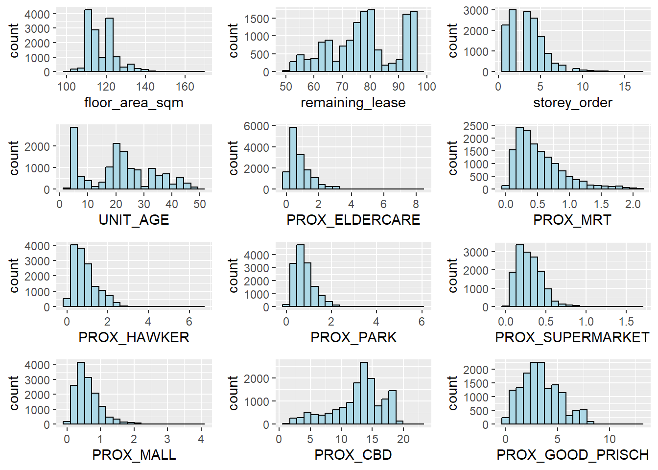
We can observe a generally right skewed nature of the above variables.
NUM_KG <- ggplot(data=train, aes(x= `WITHIN_350M_KINDERGARTEN`)) +
geom_histogram(bins=20, color="black", fill="light blue")
NUM_CC <- ggplot(data=train, aes(x= `WITHIN_350M_CHILDCARE`)) +
geom_histogram(bins=20, color="black", fill="light blue")
NUM_BUS <- ggplot(data=train, aes(x= `WITHIN_350M_BUS`)) +
geom_histogram(bins=20, color="black", fill="light blue")
NUM_PRISCH <- ggplot(data=train, aes(x= `WITHIN_1KM_PRISCH`)) +
geom_histogram(bins=20, color="black", fill="light blue")
ggarrange(NUM_KG, NUM_CC, NUM_BUS, NUM_PRISCH, ncol= 2, nrow= 2)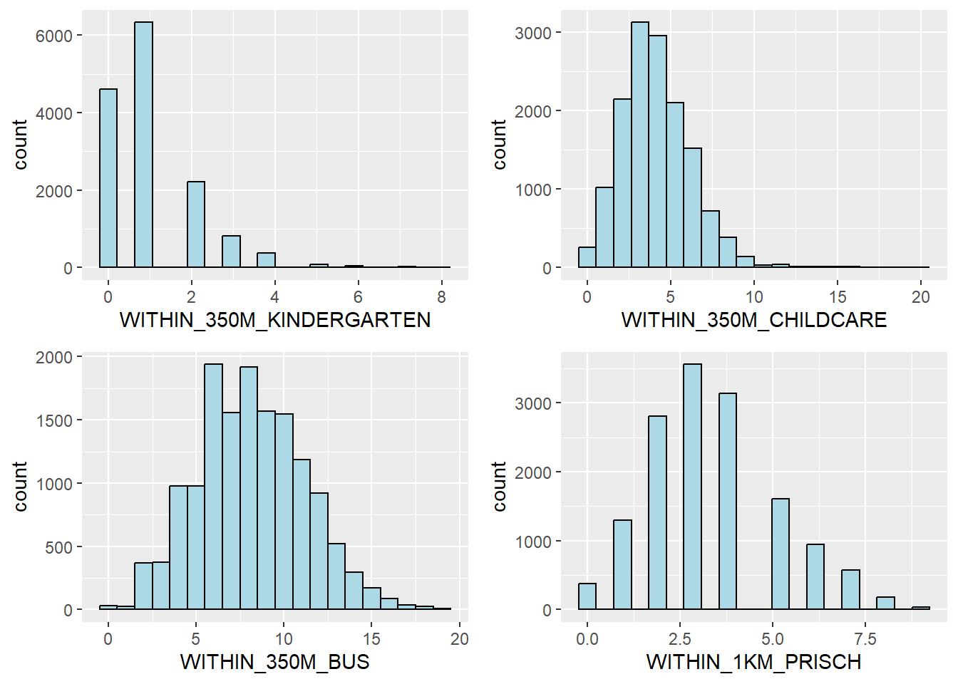
We can observe the right skewed data from ‘WITHIN_350M_KINDERGARTEN’, while the other 3 factors indicate normally distributed childcare, bus stops and primary schools.
7.2 Statistical Point Map
tmap_mode("view")tmap_options(check.and.fix = TRUE)Reading layer `MPSZ-2019' from data source
`C:\annatrw\IS415\Take-home_Ex\Take-home_Ex03\data\geospatial\MPSZ2019'
using driver `ESRI Shapefile'
Simple feature collection with 332 features and 6 fields
Geometry type: MULTIPOLYGON
Dimension: XY
Bounding box: xmin: 103.6057 ymin: 1.158699 xmax: 104.0885 ymax: 1.470775
Geodetic CRS: WGS 84tm_shape(mpsz_sf)+
tm_polygons() +
tm_shape(train) +
tm_dots(col = "resale_price",
alpha = 0.6,
style="quantile") +
tm_view(set.zoom.limits = c(11, 12))tmap_mode("plot")We can observe that the HDB resale prices are high in the CBD, Southern and central areas of Singapore, reaching to $720,000 to $1,418,000 range. Resale flats in the North East (Punggol, Sengkang etc) are beginning to get more expensive, reaching the $625,000 range. The West and Northern districts have a larger majority of cheaper resale HDB flats that are in the $350,000 to $625,000 range.
8 Hedonic Pricing Model
Before we begin building the pricing model for HDB resale prices, we will use the package corrplot to check for multicolinearity. The code chunk below drops the geometry field to plot correlation matrix. It uses the ‘AOE’ order, ordering variables by the eigenvectors method suggested by Michael Friendly.
train_nogeom <- train %>% st_drop_geometry()
corrplot(cor(train_nogeom[, 2:17]), diag = FALSE, order = "AOE",
tl.pos = "td", tl.cex = 0.5, method = "number", type = "upper")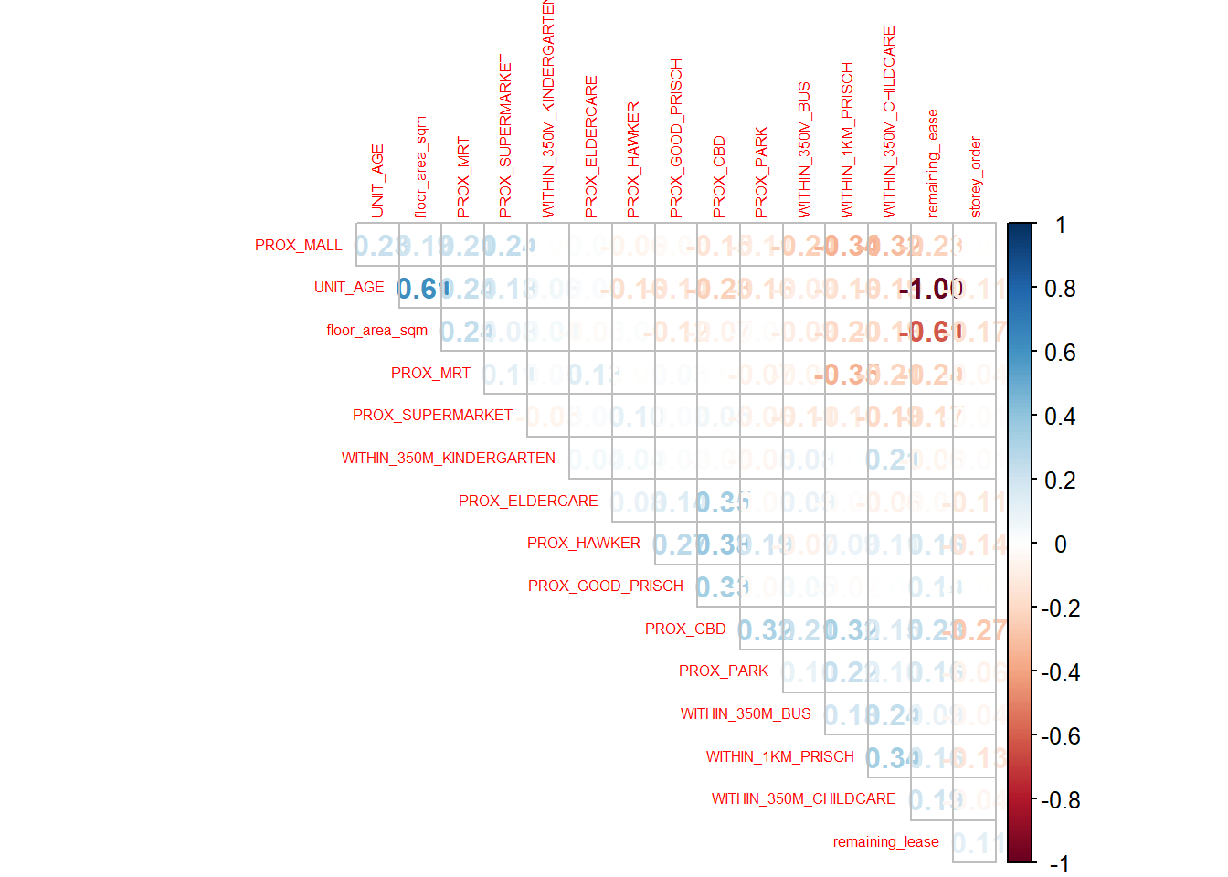
The correlation matrix above shows that all values are below 0.8 apart from UNIT_AGE and remaining_lease that has a value of 1, indicating they are highly correlated.
Therefore, the UNIT_AGE variable will be excluded from subsequent analysis.
train <- subset(train, select= -c(UNIT_AGE))test <- subset(test, select= -c(UNIT_AGE))8.1 Ordinary Least Squares (OLS) Method
Compute the regression model using the lm() function below.
train_nogeom <- train %>% st_drop_geometry()
price_mlr <- lm(resale_price ~ .,
data=train_nogeom)
summary(price_mlr)
Call:
lm(formula = resale_price ~ ., data = train_nogeom)
Residuals:
Min 1Q Median 3Q Max
-324299 -54097 -2735 48780 715869
Coefficients:
Estimate Std. Error t value Pr(>|t|)
(Intercept) -165691.0 19744.8 -8.392 < 2e-16 ***
floor_area_sqm 5530.3 126.6 43.675 < 2e-16 ***
remaining_lease 5588.6 79.5 70.295 < 2e-16 ***
storey_order 19992.5 352.5 56.723 < 2e-16 ***
PROX_ELDERCARE 1002.0 1180.4 0.849 0.39595
PROX_MRT -25078.5 2016.2 -12.439 < 2e-16 ***
PROX_HAWKER -32340.1 1382.1 -23.399 < 2e-16 ***
PROX_PARK 7980.0 1752.5 4.554 5.32e-06 ***
PROX_SUPERMARKET -8458.9 4651.4 -1.819 0.06900 .
PROX_MALL -23894.5 2090.7 -11.429 < 2e-16 ***
WITHIN_350M_KINDERGARTEN 8418.9 668.8 12.588 < 2e-16 ***
WITHIN_350M_CHILDCARE -3877.4 390.7 -9.924 < 2e-16 ***
WITHIN_350M_BUS 534.2 245.4 2.177 0.02952 *
PROX_CBD -19925.7 239.9 -83.054 < 2e-16 ***
WITHIN_1KM_PRISCH -14105.9 502.4 -28.078 < 2e-16 ***
PROX_GOOD_PRISCH -1322.9 418.2 -3.163 0.00156 **
---
Signif. codes: 0 '***' 0.001 '**' 0.01 '*' 0.05 '.' 0.1 ' ' 1
Residual standard error: 83390 on 14503 degrees of freedom
Multiple R-squared: 0.6746, Adjusted R-squared: 0.6742
F-statistic: 2004 on 15 and 14503 DF, p-value: < 2.2e-168.1.1 Publication Quality Table
Using gt summary package, it produces a summary table for the OLS model output for HDB resale price data.
tbl_regression(price_mlr, intercept = TRUE) %>%
add_glance_source_note(
label = list(sigma ~ "\U03C3"),
include = c(r.squared, adj.r.squared,
AIC, statistic,
p.value, sigma))| Characteristic | Beta | 95% CI1 | p-value |
|---|---|---|---|
| (Intercept) | -165,691 | -204,393, -126,989 | <0.001 |
| floor_area_sqm | 5,530 | 5,282, 5,778 | <0.001 |
| remaining_lease | 5,589 | 5,433, 5,744 | <0.001 |
| storey_order | 19,992 | 19,302, 20,683 | <0.001 |
| PROX_ELDERCARE | 1,002 | -1,312, 3,316 | 0.4 |
| PROX_MRT | -25,079 | -29,030, -21,127 | <0.001 |
| PROX_HAWKER | -32,340 | -35,049, -29,631 | <0.001 |
| PROX_PARK | 7,980 | 4,545, 11,415 | <0.001 |
| PROX_SUPERMARKET | -8,459 | -17,576, 658 | 0.069 |
| PROX_MALL | -23,894 | -27,993, -19,796 | <0.001 |
| WITHIN_350M_KINDERGARTEN | 8,419 | 7,108, 9,730 | <0.001 |
| WITHIN_350M_CHILDCARE | -3,877 | -4,643, -3,112 | <0.001 |
| WITHIN_350M_BUS | 534 | 53, 1,015 | 0.030 |
| PROX_CBD | -19,926 | -20,396, -19,455 | <0.001 |
| WITHIN_1KM_PRISCH | -14,106 | -15,091, -13,121 | <0.001 |
| PROX_GOOD_PRISCH | -1,323 | -2,143, -503 | 0.002 |
| R² = 0.675; Adjusted R² = 0.674; AIC = 370,258; Statistic = 2,004; p-value = <0.001; σ = 83,388 | |||
| 1 CI = Confidence Interval | |||
8.1.2 Check Non-linearity
ols_plot_resid_fit(price_mlr)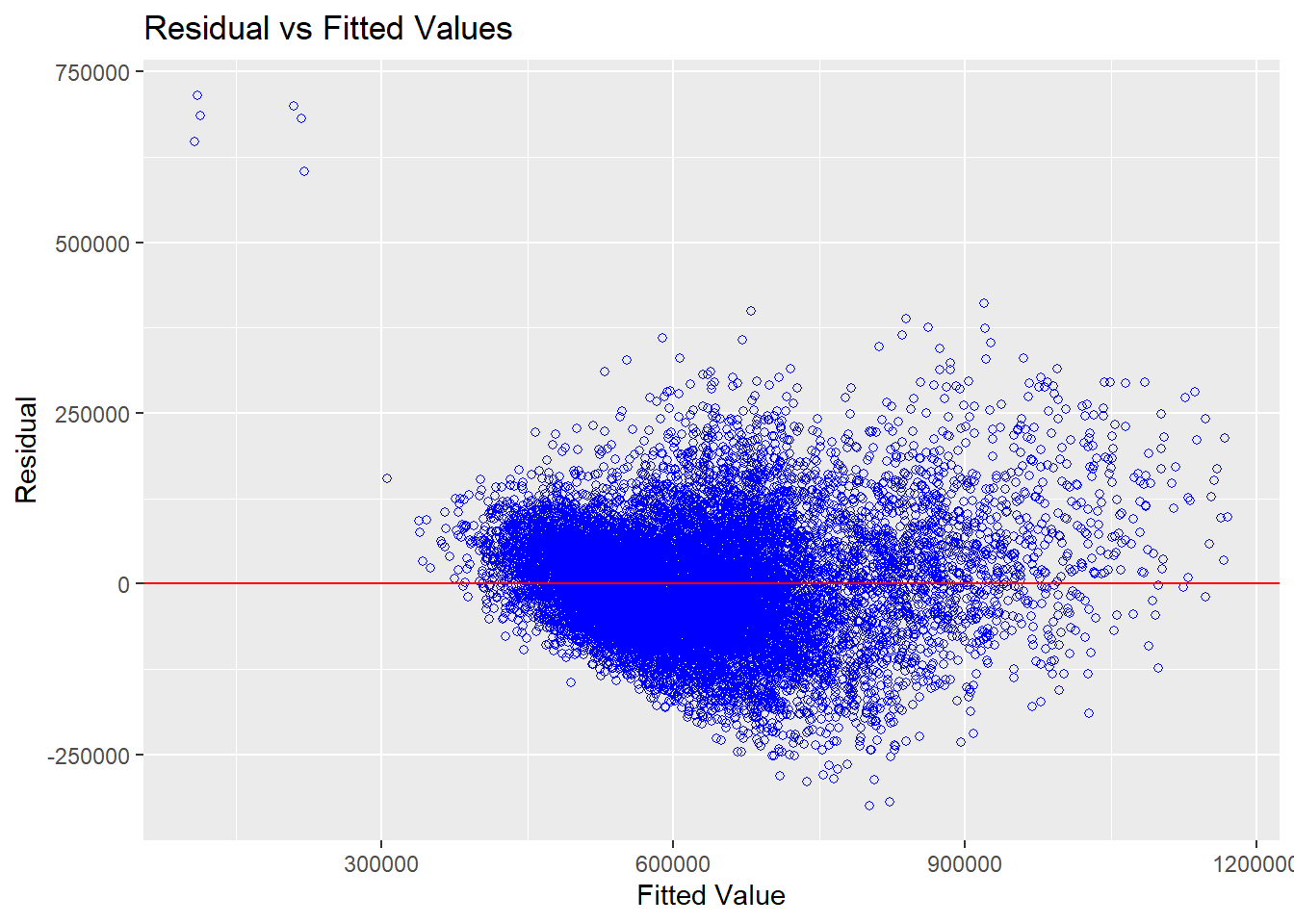
The points are scattered around 0 line, indicating that the dependent variable (price) and independent variables have a linear relationship.
8.1.3 Check Multicolinearity
vif <- ols_vif_tol(price_mlr)
vif Variables Tolerance VIF
1 floor_area_sqm 0.5598668 1.786139
2 remaining_lease 0.5253518 1.903486
3 storey_order 0.8703427 1.148973
4 PROX_ELDERCARE 0.8084843 1.236882
5 PROX_MRT 0.8038367 1.244034
6 PROX_HAWKER 0.7643724 1.308263
7 PROX_PARK 0.8262207 1.210330
8 PROX_SUPERMARKET 0.8722162 1.146505
9 PROX_MALL 0.7694176 1.299684
10 WITHIN_350M_KINDERGARTEN 0.9239515 1.082308
11 WITHIN_350M_CHILDCARE 0.7381697 1.354702
12 WITHIN_350M_BUS 0.8500367 1.176420
13 PROX_CBD 0.5009505 1.996205
14 WITHIN_1KM_PRISCH 0.6576783 1.520500
15 PROX_GOOD_PRISCH 0.8104372 1.233902We can observe that all vif values are well below 5, indicating there is no multicolinearity between the independent variables.
8.1.4 Check Normality Assumption
From the ols_plot_resid_hist package, the residuals are resembling a normal distribution.
ols_plot_resid_hist(price_mlr)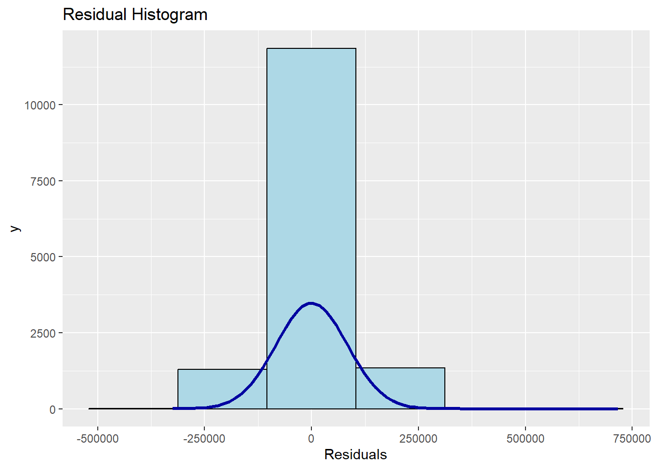
8.1.5 Check Spatial Autocorrelation
Since we are building a predictive geographically weighted regression model that accounts for spatial distribution, we check for spatial autocorrelation to understand the relationship data points have with neighbouring points.
Extract out the residuals and convert it into a dataframe.
mlr.output <- as.data.frame(price_mlr$residuals)
price_resale.res.sf <- cbind(train,
price_mlr$residuals) %>%
rename(`MLR_RES` = `price_mlr.residuals`)Next, convert it into an sp spatial object to prepare the residuals for the spatial autocorrelation test.
price_resale.sp <- as_Spatial(price_resale.res.sf)
price_resale.spclass : SpatialPointsDataFrame
features : 14519
extent : 6958.193, 42645.18, 28157.26, 48741.06 (xmin, xmax, ymin, ymax)
crs : +proj=tmerc +lat_0=1.36666666666667 +lon_0=103.833333333333 +k=1 +x_0=28001.642 +y_0=38744.572 +ellps=WGS84 +towgs84=0,0,0,0,0,0,0 +units=m +no_defs
variables : 17
names : resale_price, floor_area_sqm, remaining_lease, storey_order, PROX_ELDERCARE, PROX_MRT, PROX_HAWKER, PROX_PARK, PROX_SUPERMARKET, PROX_MALL, WITHIN_350M_KINDERGARTEN, WITHIN_350M_CHILDCARE, WITHIN_350M_BUS, PROX_CBD, WITHIN_1KM_PRISCH, ...
min values : 350000, 99, 49.08, 1, 3.24852165967354e-07, 0.0229291315265009, 0.0494878683203785, 0.0600396043825887, 7.47984318619627e-07, 2.21189111471176e-12, 0, 0, 0, 1.6109563636452, 0, ...
max values : 1418000, 167, 96.75, 17, 8.26597091415839, 2.12908590009577, 6.63382585101601, 6.00301683925507, 1.67131003223853, 4.00920093399656, 8, 20, 19, 23.2773731998479, 9, ... tmap_mode("view")tm_shape(mpsz_sf)+
tmap_options(check.and.fix = TRUE) +
tm_polygons(alpha = 0.4) +
tm_shape(price_resale.res.sf) +
tm_dots(col = "MLR_RES",
alpha = 0.6,
style="quantile") +
tm_view(set.zoom.limits = c(11,14))tmap_mode("plot")From the tmap plot of residuals, we can observe signs of spatial clustering, hence we can perform Moran I test to confirm this.
Using the dnearneigh function from spdep package, the following code chunk identifies neighbours that are euclidean distance away between the lower and upper bounds specified.
nb <- dnearneigh(coordinates(price_resale.sp), 0, 1500, longlat = FALSE)
summary(nb)Neighbour list object:
Number of regions: 14519
Number of nonzero links: 10417942
Percentage nonzero weights: 4.942066
Average number of links: 717.5385
Link number distribution:
4 5 6 13 21 29 30 32 54 55 56 57 59 62 64 67
5 6 6 8 6 6 3 7 14 52 2 4 2 2 10 2
71 72 73 74 81 84 85 86 88 89 90 91 92 93 94 95
1 3 2 1 6 8 9 1 6 13 5 11 5 7 2 11
96 98 99 100 101 102 103 104 105 106 108 109 111 113 114 115
21 3 11 17 1 5 10 8 5 4 8 4 6 10 12 23
116 117 118 119 120 121 122 123 124 125 126 127 128 129 131 132
9 6 16 5 32 4 4 11 10 16 4 23 134 44 38 7
133 134 135 136 137 138 139 140 141 142 143 144 145 146 147 148
4 17 16 12 5 10 16 1 1 8 13 28 9 8 4 10
149 150 151 152 153 154 155 156 157 158 159 160 161 162 163 166
10 16 24 11 6 11 57 5 12 3 26 11 24 8 16 6
167 168 170 171 172 173 174 175 176 177 178 179 180 181 182 183
13 21 10 24 12 11 5 4 18 11 3 18 12 12 6 1
184 185 186 187 188 189 190 191 192 193 194 195 197 198 199 200
31 15 4 23 33 3 5 3 9 26 3 16 27 1 2 6
201 202 203 204 205 206 207 208 209 210 211 212 213 214 215 216
14 1 10 10 6 3 14 13 14 16 17 13 16 14 11 15
217 218 219 220 221 222 223 224 225 226 227 228 229 230 231 232
14 8 3 29 18 12 48 16 13 4 14 3 3 6 20 23
233 234 235 236 237 238 239 240 241 242 243 244 245 246 247 248
6 8 44 30 5 12 18 34 32 19 6 8 7 5 11 5
249 250 251 252 253 254 255 256 257 258 259 260 261 262 263 264
6 17 6 8 54 1 8 7 4 3 6 25 8 1 25 3
265 266 267 268 269 270 271 272 273 274 275 276 277 278 279 280
11 17 4 17 21 12 12 31 15 6 29 26 20 49 47 16
281 282 283 284 285 286 287 288 289 290 291 292 293 294 295 296
4 11 10 21 20 6 23 14 27 15 16 14 41 10 10 12
297 298 299 300 301 302 303 304 305 306 307 308 309 310 311 312
22 34 16 21 19 24 15 24 15 4 21 18 8 20 9 33
313 314 315 316 317 318 319 320 321 322 323 324 325 326 327 328
13 2 26 16 14 18 6 21 18 18 6 25 47 5 25 15
329 330 331 332 333 334 335 336 337 338 339 340 341 342 343 344
19 27 38 22 35 38 38 24 16 78 43 23 21 42 46 26
345 346 347 348 349 350 351 352 353 354 355 356 357 358 359 360
32 6 33 37 27 13 14 7 14 16 31 21 18 13 16 25
361 362 363 364 365 366 367 368 369 370 372 373 374 375 376 377
23 49 11 1 6 20 17 38 16 23 17 11 36 17 7 4
378 379 380 381 382 383 384 385 386 387 388 389 390 391 392 393
13 4 19 17 14 6 12 5 53 27 6 31 27 20 4 46
394 395 396 397 398 399 400 401 402 403 404 405 406 407 408 409
30 6 31 1 20 3 8 23 26 11 23 38 8 17 4 20
410 411 412 413 414 415 416 417 418 419 420 421 422 423 424 425
45 18 13 22 20 28 15 16 9 11 13 23 24 48 3 22
426 427 428 429 430 431 432 433 434 435 436 437 438 439 440 441
8 21 20 49 21 25 17 6 6 10 40 14 12 38 4 10
442 443 444 445 446 447 448 449 450 451 452 453 454 455 456 457
9 25 8 26 7 30 10 11 17 17 20 34 12 22 11 13
458 459 460 461 462 463 464 465 466 467 468 469 470 471 472 473
13 17 17 8 37 17 6 14 8 25 20 13 2 13 14 7
474 475 476 477 478 479 480 481 482 483 484 485 486 487 488 489
2 10 20 15 10 19 20 6 11 25 19 6 10 12 8 13
490 491 492 493 494 495 496 497 498 499 500 501 502 503 504 505
20 13 6 17 6 23 9 5 28 6 6 30 16 25 36 20
506 507 508 509 510 511 512 513 514 515 516 517 518 519 520 521
6 29 7 3 9 14 1 7 23 2 20 12 16 6 11 33
522 523 524 525 526 527 528 529 530 531 532 533 534 535 536 537
12 26 8 5 31 9 7 10 17 10 14 10 14 15 32 5
538 539 540 542 543 544 545 547 548 549 550 551 553 554 555 556
5 19 22 14 11 1 14 4 10 10 11 16 10 5 28 4
557 558 559 560 561 562 563 564 565 566 567 568 569 570 571 572
7 14 21 8 9 6 6 2 5 11 8 12 4 36 20 1
573 574 575 576 577 578 579 580 581 582 583 584 585 586 587 588
13 6 29 4 13 7 6 10 16 7 23 3 17 10 31 17
589 590 591 592 593 595 596 597 598 599 600 601 602 603 604 605
8 13 8 3 19 7 21 8 11 19 9 28 1 19 10 20
606 607 608 609 610 611 612 613 614 615 616 617 618 619 620 621
1 21 16 14 14 6 17 16 17 22 21 10 28 33 40 45
622 623 624 625 626 627 628 629 630 631 632 633 634 635 636 637
22 11 12 14 44 27 16 2 18 56 24 9 12 15 23 33
638 639 640 641 642 643 644 645 646 647 648 649 650 651 652 653
46 20 6 25 21 15 23 8 8 18 12 16 11 10 4 27
654 655 656 657 658 659 660 661 662 663 664 665 666 667 668 669
21 16 24 13 13 19 25 18 7 15 6 6 25 2 20 14
670 671 672 673 674 675 676 677 678 679 680 682 683 684 685 686
8 34 2 10 9 35 31 6 7 13 19 5 7 4 51 15
687 688 689 691 692 693 694 695 696 697 698 699 700 701 702 703
10 9 20 5 31 6 29 9 18 19 26 11 9 5 13 13
704 705 707 708 709 710 711 712 713 714 715 716 717 718 719 720
3 25 10 14 8 10 26 19 23 32 46 70 2 18 9 16
721 722 723 724 725 726 727 728 729 730 731 732 733 734 735 736
6 18 15 8 11 1 16 20 14 13 14 10 34 3 11 22
737 738 739 740 741 742 743 744 745 746 747 748 749 750 751 752
13 11 3 6 8 8 8 8 27 4 11 35 27 8 32 4
753 754 755 756 757 758 759 760 761 762 763 764 765 766 767 768
1 12 2 8 17 1 14 3 1 8 3 14 16 8 10 6
769 770 771 772 773 774 775 776 777 778 779 780 781 782 783 784
7 33 19 15 6 3 4 22 3 10 9 3 1 9 11 3
785 786 787 788 789 790 791 792 793 794 795 796 797 798 799 800
4 7 26 3 3 8 6 17 1 8 2 10 13 12 1 2
801 802 803 804 805 806 807 808 809 810 811 813 815 819 820 821
8 2 6 4 8 1 7 4 8 5 12 5 10 8 11 4
823 824 827 828 829 830 831 832 833 834 835 838 839 840 842 843
3 3 7 3 1 7 4 4 1 6 1 12 7 1 3 16
845 846 847 848 849 850 852 854 856 857 858 861 862 863 865 866
3 1 4 3 4 8 3 6 11 1 5 4 2 4 3 4
867 868 870 871 872 873 874 875 878 879 880 883 884 885 889 890
11 5 2 1 3 1 3 7 7 3 3 1 6 1 4 10
892 893 894 896 897 898 899 900 901 903 904 907 908 909 910 912
5 7 1 4 4 1 2 4 10 4 7 10 5 1 2 7
913 914 929 933 935 942 949 950 964 967 971 973 985 997 1001 1006
10 21 6 3 1 5 6 3 1 11 6 1 34 10 8 8
1009 1022 1026 1027 1030 1040 1045 1051 1054 1079 1092 1093 1095 1097 1101 1102
2 17 7 3 12 10 17 2 1 15 5 13 34 8 6 6
1120 1124 1132 1137 1144 1148 1151 1152 1156 1160 1167 1170 1173 1175 1183 1186
7 2 7 2 3 10 4 19 12 7 3 3 2 22 3 2
1195 1199 1204 1212 1217 1220 1223 1226 1239 1243 1247 1250 1252 1254 1259 1261
12 21 7 1 4 5 38 16 4 8 2 1 5 2 7 4
1263 1264 1266 1267 1268 1273 1276 1280 1285 1291 1292 1294 1295 1296 1297 1298
3 3 1 5 3 5 7 36 1 5 11 8 7 3 4 2
1300 1305 1309 1313 1316 1317 1320 1324 1333 1335 1336 1344 1348 1352 1354 1356
3 5 4 8 1 4 9 3 4 2 3 5 5 11 3 5
1357 1359 1364 1366 1367 1368 1369 1379 1383 1384 1390 1392 1396 1399 1401 1402
7 6 10 2 4 4 4 4 12 4 11 17 7 5 2 13
1403 1405 1407 1408 1410 1411 1413 1415 1416 1417 1422 1423 1424 1426 1429 1431
9 5 10 4 8 8 6 5 10 1 3 3 17 9 8 12
1432 1433 1435 1436 1437 1438 1441 1442 1444 1447 1448 1451 1453 1455 1456 1458
6 4 4 11 11 7 9 6 2 5 4 10 9 20 6 16
1462 1463 1464 1467 1472 1474 1479 1482 1483 1486 1487 1489 1492 1493 1496 1497
8 15 12 8 10 3 20 5 8 5 8 16 3 9 4 6
1498 1499 1501 1506 1510 1513 1514 1519 1524 1525 1526 1528 1529 1531 1532 1533
7 7 3 12 4 8 3 2 2 4 13 3 3 10 3 42
1534 1535 1538 1539 1540 1541 1542 1543 1544 1545 1548 1549 1550 1551 1552 1556
15 7 5 9 16 6 2 9 5 2 3 4 12 4 3 2
1557 1558 1559 1561 1562 1565 1566 1568 1569 1572 1573 1577 1579 1580 1583 1584
4 8 9 4 1 2 2 18 20 8 5 8 9 4 5 2
1586 1587 1589 1590 1598 1600 1601 1603 1609 1610 1611 1612 1615 1616 1617 1620
5 16 5 14 1 3 7 2 5 9 5 13 11 25 13 2
1624 1629 1633 1635 1636 1638 1641 1642 1647 1648 1650 1652 1654 1655 1656 1657
7 7 9 4 3 17 11 4 5 6 6 13 3 5 12 6
1658 1660 1661 1662 1666 1667 1668 1671 1676 1679 1682 1683 1684 1685 1689 1690
7 9 14 9 2 9 15 6 4 6 4 3 3 17 9 1
1691 1692 1694 1707 1709 1712 1713 1717 1718 1719 1720 1721 1730 1731 1732 1734
2 8 4 15 12 7 2 2 6 3 12 6 1 11 7 8
1736 1738 1739 1741 1743 1744 1745 1746 1747 1759 1762 1765 1771 1773 1775 1786
8 5 12 3 6 12 8 7 10 5 2 4 3 1 2 10
1794 1803 1805 1808 1810 1813 1815 1817 1821 1823 1828 1831 1832 1844 1853 1856
18 3 3 11 6 7 1 2 8 8 9 3 1 5 4 2
1862 1865 1871 1878 1880 1883 1884 1886 1888 1889 1891 1892 1893 1898 1902 1907
4 6 7 14 2 4 7 5 8 3 9 6 9 4 2 2
1909 1910 1920 1921 1924 1933 1935 1937 1938 1940 1941 1942 1945 1949 1952 1955
5 11 6 2 2 6 3 1 2 4 1 6 7 2 6 2
1959 1961 1964 1965 1969 1974 1976 1977 1980 1988 1991 1993 1996 1999 2005 2010
5 3 4 4 3 3 10 4 6 3 5 9 3 12 6 5
2012 2014 2017 2024 2027 2029 2033 2036 2042 2043 2045 2046 2052 2053 2055 2061
5 4 7 15 4 15 9 4 1 2 5 3 5 13 1 19
2063 2066 2067 2069 2071 2077 2081 2084 2092 2093 2097 2098 2100 2109 2110 2112
15 2 1 6 6 6 9 1 6 3 2 6 2 12 15 11
2115 2117 2118 2119 2138 2142 2143 2145 2148 2154 2158 2164 2165 2170 2171 2172
3 2 3 2 8 1 2 15 1 4 1 10 3 4 2 6
2186 2188 2190 2194 2198 2200 2204 2208 2216 2218 2227 2229 2233 2236 2237 2240
4 4 6 2 5 8 5 16 2 9 6 4 4 5 3 8
2244 2245 2248 2249 2251 2253 2256 2260 2263 2264 2265 2275 2276 2280 2290 2303
3 4 3 3 5 5 3 13 1 10 6 2 4 11 2 4
2304 2305 2306 2310 2313 2314 2316 2317 2319 2320 2321 2322 2326 2327 2335 2338
5 7 5 4 3 8 6 4 4 2 2 4 2 5 5 4
2345 2346 2347 2350 2351 2354 2356 2358 2372 2375 2378 2387 2388 2392 2393 2398
6 2 3 5 7 1 2 3 4 5 4 7 5 5 1 4
2403 2404 2406 2407 2409 2412 2413 2417 2418 2419 2426 2430 2431 2434 2435 2439
4 1 5 5 4 1 5 5 2 4 4 10 5 7 5 6
2444 2445 2457 2462 2464 2474 2479 2490 2493 2494 2496 2502 2508 2509 2516 2517
6 1 2 7 6 4 8 7 15 8 4 5 1 11 2 5
2519 2552
2 5
5 least connected regions:
918 6125 10704 10705 10706 with 4 links
5 most connected regions:
4165 6296 6974 7602 12525 with 2552 linksThe next code chunk below converts the neighbours list into spatial weights using nb2listw function.
nb_lw <- nb2listw(nb, style = 'W')
summary(nb_lw)Characteristics of weights list object:
Neighbour list object:
Number of regions: 14519
Number of nonzero links: 10417942
Percentage nonzero weights: 4.942066
Average number of links: 717.5385
Link number distribution:
4 5 6 13 21 29 30 32 54 55 56 57 59 62 64 67
5 6 6 8 6 6 3 7 14 52 2 4 2 2 10 2
71 72 73 74 81 84 85 86 88 89 90 91 92 93 94 95
1 3 2 1 6 8 9 1 6 13 5 11 5 7 2 11
96 98 99 100 101 102 103 104 105 106 108 109 111 113 114 115
21 3 11 17 1 5 10 8 5 4 8 4 6 10 12 23
116 117 118 119 120 121 122 123 124 125 126 127 128 129 131 132
9 6 16 5 32 4 4 11 10 16 4 23 134 44 38 7
133 134 135 136 137 138 139 140 141 142 143 144 145 146 147 148
4 17 16 12 5 10 16 1 1 8 13 28 9 8 4 10
149 150 151 152 153 154 155 156 157 158 159 160 161 162 163 166
10 16 24 11 6 11 57 5 12 3 26 11 24 8 16 6
167 168 170 171 172 173 174 175 176 177 178 179 180 181 182 183
13 21 10 24 12 11 5 4 18 11 3 18 12 12 6 1
184 185 186 187 188 189 190 191 192 193 194 195 197 198 199 200
31 15 4 23 33 3 5 3 9 26 3 16 27 1 2 6
201 202 203 204 205 206 207 208 209 210 211 212 213 214 215 216
14 1 10 10 6 3 14 13 14 16 17 13 16 14 11 15
217 218 219 220 221 222 223 224 225 226 227 228 229 230 231 232
14 8 3 29 18 12 48 16 13 4 14 3 3 6 20 23
233 234 235 236 237 238 239 240 241 242 243 244 245 246 247 248
6 8 44 30 5 12 18 34 32 19 6 8 7 5 11 5
249 250 251 252 253 254 255 256 257 258 259 260 261 262 263 264
6 17 6 8 54 1 8 7 4 3 6 25 8 1 25 3
265 266 267 268 269 270 271 272 273 274 275 276 277 278 279 280
11 17 4 17 21 12 12 31 15 6 29 26 20 49 47 16
281 282 283 284 285 286 287 288 289 290 291 292 293 294 295 296
4 11 10 21 20 6 23 14 27 15 16 14 41 10 10 12
297 298 299 300 301 302 303 304 305 306 307 308 309 310 311 312
22 34 16 21 19 24 15 24 15 4 21 18 8 20 9 33
313 314 315 316 317 318 319 320 321 322 323 324 325 326 327 328
13 2 26 16 14 18 6 21 18 18 6 25 47 5 25 15
329 330 331 332 333 334 335 336 337 338 339 340 341 342 343 344
19 27 38 22 35 38 38 24 16 78 43 23 21 42 46 26
345 346 347 348 349 350 351 352 353 354 355 356 357 358 359 360
32 6 33 37 27 13 14 7 14 16 31 21 18 13 16 25
361 362 363 364 365 366 367 368 369 370 372 373 374 375 376 377
23 49 11 1 6 20 17 38 16 23 17 11 36 17 7 4
378 379 380 381 382 383 384 385 386 387 388 389 390 391 392 393
13 4 19 17 14 6 12 5 53 27 6 31 27 20 4 46
394 395 396 397 398 399 400 401 402 403 404 405 406 407 408 409
30 6 31 1 20 3 8 23 26 11 23 38 8 17 4 20
410 411 412 413 414 415 416 417 418 419 420 421 422 423 424 425
45 18 13 22 20 28 15 16 9 11 13 23 24 48 3 22
426 427 428 429 430 431 432 433 434 435 436 437 438 439 440 441
8 21 20 49 21 25 17 6 6 10 40 14 12 38 4 10
442 443 444 445 446 447 448 449 450 451 452 453 454 455 456 457
9 25 8 26 7 30 10 11 17 17 20 34 12 22 11 13
458 459 460 461 462 463 464 465 466 467 468 469 470 471 472 473
13 17 17 8 37 17 6 14 8 25 20 13 2 13 14 7
474 475 476 477 478 479 480 481 482 483 484 485 486 487 488 489
2 10 20 15 10 19 20 6 11 25 19 6 10 12 8 13
490 491 492 493 494 495 496 497 498 499 500 501 502 503 504 505
20 13 6 17 6 23 9 5 28 6 6 30 16 25 36 20
506 507 508 509 510 511 512 513 514 515 516 517 518 519 520 521
6 29 7 3 9 14 1 7 23 2 20 12 16 6 11 33
522 523 524 525 526 527 528 529 530 531 532 533 534 535 536 537
12 26 8 5 31 9 7 10 17 10 14 10 14 15 32 5
538 539 540 542 543 544 545 547 548 549 550 551 553 554 555 556
5 19 22 14 11 1 14 4 10 10 11 16 10 5 28 4
557 558 559 560 561 562 563 564 565 566 567 568 569 570 571 572
7 14 21 8 9 6 6 2 5 11 8 12 4 36 20 1
573 574 575 576 577 578 579 580 581 582 583 584 585 586 587 588
13 6 29 4 13 7 6 10 16 7 23 3 17 10 31 17
589 590 591 592 593 595 596 597 598 599 600 601 602 603 604 605
8 13 8 3 19 7 21 8 11 19 9 28 1 19 10 20
606 607 608 609 610 611 612 613 614 615 616 617 618 619 620 621
1 21 16 14 14 6 17 16 17 22 21 10 28 33 40 45
622 623 624 625 626 627 628 629 630 631 632 633 634 635 636 637
22 11 12 14 44 27 16 2 18 56 24 9 12 15 23 33
638 639 640 641 642 643 644 645 646 647 648 649 650 651 652 653
46 20 6 25 21 15 23 8 8 18 12 16 11 10 4 27
654 655 656 657 658 659 660 661 662 663 664 665 666 667 668 669
21 16 24 13 13 19 25 18 7 15 6 6 25 2 20 14
670 671 672 673 674 675 676 677 678 679 680 682 683 684 685 686
8 34 2 10 9 35 31 6 7 13 19 5 7 4 51 15
687 688 689 691 692 693 694 695 696 697 698 699 700 701 702 703
10 9 20 5 31 6 29 9 18 19 26 11 9 5 13 13
704 705 707 708 709 710 711 712 713 714 715 716 717 718 719 720
3 25 10 14 8 10 26 19 23 32 46 70 2 18 9 16
721 722 723 724 725 726 727 728 729 730 731 732 733 734 735 736
6 18 15 8 11 1 16 20 14 13 14 10 34 3 11 22
737 738 739 740 741 742 743 744 745 746 747 748 749 750 751 752
13 11 3 6 8 8 8 8 27 4 11 35 27 8 32 4
753 754 755 756 757 758 759 760 761 762 763 764 765 766 767 768
1 12 2 8 17 1 14 3 1 8 3 14 16 8 10 6
769 770 771 772 773 774 775 776 777 778 779 780 781 782 783 784
7 33 19 15 6 3 4 22 3 10 9 3 1 9 11 3
785 786 787 788 789 790 791 792 793 794 795 796 797 798 799 800
4 7 26 3 3 8 6 17 1 8 2 10 13 12 1 2
801 802 803 804 805 806 807 808 809 810 811 813 815 819 820 821
8 2 6 4 8 1 7 4 8 5 12 5 10 8 11 4
823 824 827 828 829 830 831 832 833 834 835 838 839 840 842 843
3 3 7 3 1 7 4 4 1 6 1 12 7 1 3 16
845 846 847 848 849 850 852 854 856 857 858 861 862 863 865 866
3 1 4 3 4 8 3 6 11 1 5 4 2 4 3 4
867 868 870 871 872 873 874 875 878 879 880 883 884 885 889 890
11 5 2 1 3 1 3 7 7 3 3 1 6 1 4 10
892 893 894 896 897 898 899 900 901 903 904 907 908 909 910 912
5 7 1 4 4 1 2 4 10 4 7 10 5 1 2 7
913 914 929 933 935 942 949 950 964 967 971 973 985 997 1001 1006
10 21 6 3 1 5 6 3 1 11 6 1 34 10 8 8
1009 1022 1026 1027 1030 1040 1045 1051 1054 1079 1092 1093 1095 1097 1101 1102
2 17 7 3 12 10 17 2 1 15 5 13 34 8 6 6
1120 1124 1132 1137 1144 1148 1151 1152 1156 1160 1167 1170 1173 1175 1183 1186
7 2 7 2 3 10 4 19 12 7 3 3 2 22 3 2
1195 1199 1204 1212 1217 1220 1223 1226 1239 1243 1247 1250 1252 1254 1259 1261
12 21 7 1 4 5 38 16 4 8 2 1 5 2 7 4
1263 1264 1266 1267 1268 1273 1276 1280 1285 1291 1292 1294 1295 1296 1297 1298
3 3 1 5 3 5 7 36 1 5 11 8 7 3 4 2
1300 1305 1309 1313 1316 1317 1320 1324 1333 1335 1336 1344 1348 1352 1354 1356
3 5 4 8 1 4 9 3 4 2 3 5 5 11 3 5
1357 1359 1364 1366 1367 1368 1369 1379 1383 1384 1390 1392 1396 1399 1401 1402
7 6 10 2 4 4 4 4 12 4 11 17 7 5 2 13
1403 1405 1407 1408 1410 1411 1413 1415 1416 1417 1422 1423 1424 1426 1429 1431
9 5 10 4 8 8 6 5 10 1 3 3 17 9 8 12
1432 1433 1435 1436 1437 1438 1441 1442 1444 1447 1448 1451 1453 1455 1456 1458
6 4 4 11 11 7 9 6 2 5 4 10 9 20 6 16
1462 1463 1464 1467 1472 1474 1479 1482 1483 1486 1487 1489 1492 1493 1496 1497
8 15 12 8 10 3 20 5 8 5 8 16 3 9 4 6
1498 1499 1501 1506 1510 1513 1514 1519 1524 1525 1526 1528 1529 1531 1532 1533
7 7 3 12 4 8 3 2 2 4 13 3 3 10 3 42
1534 1535 1538 1539 1540 1541 1542 1543 1544 1545 1548 1549 1550 1551 1552 1556
15 7 5 9 16 6 2 9 5 2 3 4 12 4 3 2
1557 1558 1559 1561 1562 1565 1566 1568 1569 1572 1573 1577 1579 1580 1583 1584
4 8 9 4 1 2 2 18 20 8 5 8 9 4 5 2
1586 1587 1589 1590 1598 1600 1601 1603 1609 1610 1611 1612 1615 1616 1617 1620
5 16 5 14 1 3 7 2 5 9 5 13 11 25 13 2
1624 1629 1633 1635 1636 1638 1641 1642 1647 1648 1650 1652 1654 1655 1656 1657
7 7 9 4 3 17 11 4 5 6 6 13 3 5 12 6
1658 1660 1661 1662 1666 1667 1668 1671 1676 1679 1682 1683 1684 1685 1689 1690
7 9 14 9 2 9 15 6 4 6 4 3 3 17 9 1
1691 1692 1694 1707 1709 1712 1713 1717 1718 1719 1720 1721 1730 1731 1732 1734
2 8 4 15 12 7 2 2 6 3 12 6 1 11 7 8
1736 1738 1739 1741 1743 1744 1745 1746 1747 1759 1762 1765 1771 1773 1775 1786
8 5 12 3 6 12 8 7 10 5 2 4 3 1 2 10
1794 1803 1805 1808 1810 1813 1815 1817 1821 1823 1828 1831 1832 1844 1853 1856
18 3 3 11 6 7 1 2 8 8 9 3 1 5 4 2
1862 1865 1871 1878 1880 1883 1884 1886 1888 1889 1891 1892 1893 1898 1902 1907
4 6 7 14 2 4 7 5 8 3 9 6 9 4 2 2
1909 1910 1920 1921 1924 1933 1935 1937 1938 1940 1941 1942 1945 1949 1952 1955
5 11 6 2 2 6 3 1 2 4 1 6 7 2 6 2
1959 1961 1964 1965 1969 1974 1976 1977 1980 1988 1991 1993 1996 1999 2005 2010
5 3 4 4 3 3 10 4 6 3 5 9 3 12 6 5
2012 2014 2017 2024 2027 2029 2033 2036 2042 2043 2045 2046 2052 2053 2055 2061
5 4 7 15 4 15 9 4 1 2 5 3 5 13 1 19
2063 2066 2067 2069 2071 2077 2081 2084 2092 2093 2097 2098 2100 2109 2110 2112
15 2 1 6 6 6 9 1 6 3 2 6 2 12 15 11
2115 2117 2118 2119 2138 2142 2143 2145 2148 2154 2158 2164 2165 2170 2171 2172
3 2 3 2 8 1 2 15 1 4 1 10 3 4 2 6
2186 2188 2190 2194 2198 2200 2204 2208 2216 2218 2227 2229 2233 2236 2237 2240
4 4 6 2 5 8 5 16 2 9 6 4 4 5 3 8
2244 2245 2248 2249 2251 2253 2256 2260 2263 2264 2265 2275 2276 2280 2290 2303
3 4 3 3 5 5 3 13 1 10 6 2 4 11 2 4
2304 2305 2306 2310 2313 2314 2316 2317 2319 2320 2321 2322 2326 2327 2335 2338
5 7 5 4 3 8 6 4 4 2 2 4 2 5 5 4
2345 2346 2347 2350 2351 2354 2356 2358 2372 2375 2378 2387 2388 2392 2393 2398
6 2 3 5 7 1 2 3 4 5 4 7 5 5 1 4
2403 2404 2406 2407 2409 2412 2413 2417 2418 2419 2426 2430 2431 2434 2435 2439
4 1 5 5 4 1 5 5 2 4 4 10 5 7 5 6
2444 2445 2457 2462 2464 2474 2479 2490 2493 2494 2496 2502 2508 2509 2516 2517
6 1 2 7 6 4 8 7 15 8 4 5 1 11 2 5
2519 2552
2 5
5 least connected regions:
918 6125 10704 10705 10706 with 4 links
5 most connected regions:
4165 6296 6974 7602 12525 with 2552 links
Weights style: W
Weights constants summary:
n nn S0 S1 S2
W 14519 210801361 14519 80.30014 58598.26The Moran I test is performed below.
lm.morantest(price_mlr, nb_lw)
Global Moran I for regression residuals
data:
model: lm(formula = resale_price ~ ., data = train_nogeom)
weights: nb_lw
Moran I statistic standard deviate = 534.39, p-value < 2.2e-16
alternative hypothesis: greater
sample estimates:
Observed Moran I Expectation Variance
2.939151e-01 -4.904277e-04 3.035164e-07 Since the p-value is less than 2.2e-16 which is smaller than the alpha value of 0.05, there is evidence to conclude the residuals are not randomly distributed. the Observed Moran I value is 0.29395 which is larger than 0, indicating the residuals resemble a clustered distribution.
8.2 Ordinary Least Squares (OLS) Regression Predictive Model
8.2.1 Training Data
price_ols_train <- predict(price_mlr,
data=train,
se.fit = TRUE,
interval = "prediction")
summary(price_ols_train) Length Class Mode
fit 43557 -none- numeric
se.fit 14519 -none- numeric
df 1 -none- numeric
residual.scale 1 -none- numericprice_ols_train$residual.scale[1] 83388.498.2.2 Testing Data
To predict HDB resale prices using the test data, use the predict () function from the car package.
price_ols_test <- predict(price_mlr,
data=test,
se.fit = TRUE,
interval = "prediction")
summary(price_ols_test) Length Class Mode
fit 43557 -none- numeric
se.fit 14519 -none- numeric
df 1 -none- numeric
residual.scale 1 -none- numericsummary(price_ols_test$fit) fit lwr upr
Min. : 108035 Min. : -58559 Min. : 274628
1st Qu.: 542859 1st Qu.: 379321 1st Qu.: 706467
Median : 612140 Median : 448599 Median : 775661
Mean : 627297 Mean : 463755 Mean : 790839
3rd Qu.: 685101 3rd Qu.: 521575 3rd Qu.: 848660
Max. :1170458 Max. :1006807 Max. :1334109 price_ols_test$residual.scale[1] 83388.49By comparing the residuals from the training and testing data, they have yielded the same value of 83388.49, indicating that the OLS predictive model was able to predict the HDB resale prices.
8.3 Geographically Weighted Regression (GWR) Predictive Model
Convert the training data into an sp object for subsequent analysis.
train_sp <- as_Spatial(train)
train_spclass : SpatialPointsDataFrame
features : 14519
extent : 6958.193, 42645.18, 28157.26, 48741.06 (xmin, xmax, ymin, ymax)
crs : +proj=tmerc +lat_0=1.36666666666667 +lon_0=103.833333333333 +k=1 +x_0=28001.642 +y_0=38744.572 +ellps=WGS84 +towgs84=0,0,0,0,0,0,0 +units=m +no_defs
variables : 16
names : resale_price, floor_area_sqm, remaining_lease, storey_order, PROX_ELDERCARE, PROX_MRT, PROX_HAWKER, PROX_PARK, PROX_SUPERMARKET, PROX_MALL, WITHIN_350M_KINDERGARTEN, WITHIN_350M_CHILDCARE, WITHIN_350M_BUS, PROX_CBD, WITHIN_1KM_PRISCH, ...
min values : 350000, 99, 49.08, 1, 3.24852165967354e-07, 0.0229291315265009, 0.0494878683203785, 0.0600396043825887, 7.47984318619627e-07, 2.21189111471176e-12, 0, 0, 0, 1.6109563636452, 0, ...
max values : 1418000, 167, 96.75, 17, 8.26597091415839, 2.12908590009577, 6.63382585101601, 6.00301683925507, 1.67131003223853, 4.00920093399656, 8, 20, 19, 23.2773731998479, 9, ... 8.3.1 Adaptive Bandwidth
First, we will determine the optimal adaptive bandwidth for the gwr model using the code below.
bw_adaptive <- bw.gwr(resale_price ~.,
data=train_sp,
approach="CV",
kernel="gaussian",
adaptive=TRUE,
longlat=FALSE)Write the output of the optimal adaptive bandwidth into an rds file.
write_rds(bw_adaptive, "data/rds/bw_adaptive.rds") The gwr predictive model is computed below using the previously calculated optimal bandwidth:
gwr_adaptive <- gwr.basic(formula = resale_price ~
floor_area_sqm + storey_order +
remaining_lease + PROX_CBD +
PROX_ELDERCARE + PROX_HAWKER +
PROX_MRT + PROX_PARK + PROX_MALL +
PROX_SUPERMARKET + WITHIN_350M_KINDERGARTEN +
WITHIN_350M_CHILDCARE + WITHIN_350M_BUS +
WITHIN_1KM_PRISCH + PROX_GOOD_PRISCH,
data=train_sp,
bw=bw_adaptive,
kernel = 'gaussian',
adaptive=TRUE,
longlat = FALSE)Write the output of the gwr.basic model into an rds file.
write_rds(gwr_adaptive, "data/rds/gwr_adaptive.rds")Display the contents of the model below:
gwr_adaptive <- read_rds("data/rds/gwr_adaptive.rds")
gwr_adaptive ***********************************************************************
* Package GWmodel *
***********************************************************************
Program starts at: 2023-03-17 08:52:17
Call:
gwr.basic(formula = resale_price ~ floor_area_sqm + storey_order +
remaining_lease + PROX_CBD + PROX_ELDERCARE + PROX_HAWKER +
PROX_MRT + PROX_PARK + PROX_MALL + PROX_SUPERMARKET + WITHIN_350M_KINDERGARTEN +
WITHIN_350M_CHILDCARE + WITHIN_350M_BUS + WITHIN_1KM_PRISCH +
PROX_GOOD_PRISCH, data = train_sp, bw = bw_adaptive, kernel = "gaussian",
adaptive = TRUE, longlat = FALSE)
Dependent (y) variable: resale_price
Independent variables: floor_area_sqm storey_order remaining_lease PROX_CBD PROX_ELDERCARE PROX_HAWKER PROX_MRT PROX_PARK PROX_MALL PROX_SUPERMARKET WITHIN_350M_KINDERGARTEN WITHIN_350M_CHILDCARE WITHIN_350M_BUS WITHIN_1KM_PRISCH PROX_GOOD_PRISCH
Number of data points: 14519
***********************************************************************
* Results of Global Regression *
***********************************************************************
Call:
lm(formula = formula, data = data)
Residuals:
Min 1Q Median 3Q Max
-324299 -54097 -2735 48780 715869
Coefficients:
Estimate Std. Error t value Pr(>|t|)
(Intercept) -165691.0 19744.8 -8.392 < 2e-16 ***
floor_area_sqm 5530.3 126.6 43.675 < 2e-16 ***
storey_order 19992.5 352.5 56.723 < 2e-16 ***
remaining_lease 5588.6 79.5 70.295 < 2e-16 ***
PROX_CBD -19925.7 239.9 -83.054 < 2e-16 ***
PROX_ELDERCARE 1002.0 1180.4 0.849 0.39595
PROX_HAWKER -32340.1 1382.1 -23.399 < 2e-16 ***
PROX_MRT -25078.5 2016.2 -12.439 < 2e-16 ***
PROX_PARK 7980.0 1752.5 4.554 5.32e-06 ***
PROX_MALL -23894.5 2090.7 -11.429 < 2e-16 ***
PROX_SUPERMARKET -8458.9 4651.4 -1.819 0.06900 .
WITHIN_350M_KINDERGARTEN 8418.9 668.8 12.588 < 2e-16 ***
WITHIN_350M_CHILDCARE -3877.4 390.7 -9.924 < 2e-16 ***
WITHIN_350M_BUS 534.2 245.4 2.177 0.02952 *
WITHIN_1KM_PRISCH -14105.9 502.4 -28.078 < 2e-16 ***
PROX_GOOD_PRISCH -1322.9 418.2 -3.163 0.00156 **
---Significance stars
Signif. codes: 0 '***' 0.001 '**' 0.01 '*' 0.05 '.' 0.1 ' ' 1
Residual standard error: 83390 on 14503 degrees of freedom
Multiple R-squared: 0.6746
Adjusted R-squared: 0.6742
F-statistic: 2004 on 15 and 14503 DF, p-value: < 2.2e-16
***Extra Diagnostic information
Residual sum of squares: 1.008486e+14
Sigma(hat): 83348.27
AIC: 370258.4
AICc: 370258.5
BIC: 356031.2
***********************************************************************
* Results of Geographically Weighted Regression *
***********************************************************************
*********************Model calibration information*********************
Kernel function: gaussian
Adaptive bandwidth: 69 (number of nearest neighbours)
Regression points: the same locations as observations are used.
Distance metric: Euclidean distance metric is used.
****************Summary of GWR coefficient estimates:******************
Min. 1st Qu. Median 3rd Qu.
Intercept -3.7946e+08 -9.6724e+05 -1.4552e+05 3.6217e+06
floor_area_sqm -1.6034e+05 1.1165e+03 3.2034e+03 5.8176e+03
storey_order 3.3585e+03 1.1693e+04 1.4186e+04 1.7944e+04
remaining_lease -7.3105e+04 -2.1272e+03 4.0938e+03 6.6691e+03
PROX_CBD -8.8341e+07 -2.8883e+05 -2.0156e+04 9.7493e+04
PROX_ELDERCARE -1.6279e+07 -4.7141e+04 1.3052e+04 9.1405e+04
PROX_HAWKER -6.7649e+06 -5.5437e+04 3.6489e+03 1.1450e+05
PROX_MRT -7.8455e+06 -1.1892e+05 -4.9072e+04 5.2506e+04
PROX_PARK -3.5965e+07 -9.6154e+04 -1.0960e+04 6.3723e+04
PROX_MALL -2.8128e+07 -1.0545e+05 -2.3200e+04 5.9033e+04
PROX_SUPERMARKET -6.7266e+06 -9.3833e+04 -1.8712e+04 5.2123e+04
WITHIN_350M_KINDERGARTEN -3.5303e+05 -9.4771e+03 -6.3515e+02 7.4898e+03
WITHIN_350M_CHILDCARE -9.7906e+04 -3.6575e+03 4.6350e+02 5.2338e+03
WITHIN_350M_BUS -4.0644e+04 -2.6840e+03 7.9049e+01 2.7765e+03
WITHIN_1KM_PRISCH -1.5107e+06 -6.7399e+03 6.6886e+01 7.2958e+03
PROX_GOOD_PRISCH -3.8384e+07 -1.0992e+05 1.7128e+04 2.4181e+05
Max.
Intercept 791294700
floor_area_sqm 553894
storey_order 28264
remaining_lease 12809
PROX_CBD 37653414
PROX_ELDERCARE 9015002
PROX_HAWKER 36079132
PROX_MRT 13087576
PROX_PARK 12916427
PROX_MALL 15349887
PROX_SUPERMARKET 4282686
WITHIN_350M_KINDERGARTEN 222801
WITHIN_350M_CHILDCARE 62437
WITHIN_350M_BUS 25374
WITHIN_1KM_PRISCH 190039
PROX_GOOD_PRISCH 97952173
************************Diagnostic information*************************
Number of data points: 14519
Effective number of parameters (2trace(S) - trace(S'S)): 1454.963
Effective degrees of freedom (n-2trace(S) + trace(S'S)): 13064.04
AICc (GWR book, Fotheringham, et al. 2002, p. 61, eq 2.33): 353806.5
AIC (GWR book, Fotheringham, et al. 2002,GWR p. 96, eq. 4.22): 352433.6
BIC (GWR book, Fotheringham, et al. 2002,GWR p. 61, eq. 2.34): 347927.4
Residual sum of squares: 2.732835e+13
R-square value: 0.9118132
Adjusted R-square value: 0.901991
***********************************************************************
Program stops at: 2023-03-17 08:56:48 From the above output and referencing this link for interpreting GWR outputs, we can observe that the GWR model has a lower AIC value of 352433.6 compared to the Global Regression model which has a value of 370258.4, indicating that the GWR model is a better fit for the data compared to the global regression model. The Residual sum of squares for the GWR model is also smaller than that compared to the global regression model, indicating the GWR model has a closer fit to the observed data.
8.3.2 Visualise GWR output
resale.sf.adaptive <- st_as_sf(gwr_adaptive$SDF) %>%
st_transform(crs=3414)
resale.sf.adaptive.svy21 <- st_transform(resale.sf.adaptive, 3414)
resale.sf.adaptive.svy21 Simple feature collection with 14519 features and 54 fields
Geometry type: POINT
Dimension: XY
Bounding box: xmin: 6958.193 ymin: 28157.26 xmax: 42645.18 ymax: 48741.06
Projected CRS: SVY21 / Singapore TM
First 10 features:
Intercept floor_area_sqm storey_order remaining_lease PROX_CBD
1 -543922.315 5798.420 19921.33 9898.314 -858.6719
2 -455784.609 4884.513 19901.94 7705.634 2266.5729
3 -512073.474 4490.400 22228.63 7884.370 38683.0292
4 -25274.000 1843.624 24463.34 7990.419 -11223.3874
5 -626888.561 4668.305 21565.30 8089.424 42245.2023
6 1719.449 2941.478 23222.81 8571.491 -24507.6269
7 -557333.913 5302.043 19486.07 7505.329 11773.1036
8 -415412.903 4491.243 21907.71 7744.784 27745.8712
9 -337832.948 4516.634 20322.93 7771.730 -7123.5491
10 -910529.170 4195.171 21988.23 8439.962 71590.8110
PROX_ELDERCARE PROX_HAWKER PROX_MRT PROX_PARK PROX_MALL PROX_SUPERMARKET
1 -13072.20 -45495.08 -75797.72 76873.781 -93706.87 46355.87
2 -34378.12 134933.71 101221.84 -198916.246 -56710.20 -52827.67
3 -131693.52 -69535.73 51143.76 -153356.715 -114055.72 -19813.92
4 19579.72 77084.86 28637.83 -34017.472 -13903.67 20859.65
5 -172555.91 17625.06 -35577.00 -159535.592 39733.35 -47020.34
6 54207.70 10721.96 -43423.70 -6239.236 -49549.46 41126.84
7 -54903.67 171371.68 140386.22 -260819.748 -68210.93 -70784.58
8 -133868.63 -43581.03 56678.64 -164278.720 -103482.58 -47493.21
9 -37380.73 145880.12 82402.56 -211756.073 -42026.48 -55373.41
10 -168225.94 -84533.06 -86020.14 -80346.241 21808.80 84107.22
WITHIN_350M_KINDERGARTEN WITHIN_350M_CHILDCARE WITHIN_350M_BUS
1 -3702.856 4396.732 -3620.1390
2 12899.984 7369.359 8876.7757
3 10702.397 7523.916 -2211.8918
4 18586.932 -1397.015 1121.0196
5 15323.347 11072.893 2617.3135
6 20746.176 -3234.304 3210.2936
7 8886.546 8369.911 5682.4560
8 12755.269 6366.276 419.2191
9 12148.770 5232.924 8253.1675
10 -1405.150 13991.956 -2885.0542
WITHIN_1KM_PRISCH PROX_GOOD_PRISCH y yhat residual CV_Score
1 -19651.954 -14798.835 483000 520774.3 -37774.29 0
2 -22308.331 -4372.036 590000 678469.4 -88469.37 0
3 -52699.212 19801.413 629000 705712.4 -76712.40 0
4 -1117.886 -35827.116 670000 812096.3 -142096.27 0
5 -60158.652 5470.719 680000 732430.0 -52430.00 0
6 -4990.206 -47860.821 760000 847500.1 -87500.08 0
7 -23742.899 10531.956 768000 871399.0 -103398.99 0
8 -56144.137 20399.417 816800 847604.5 -30804.54 0
9 -18145.095 2667.099 820000 869514.4 -49514.42 0
10 -33729.036 22267.276 830000 931320.1 -101320.12 0
Stud_residual Intercept_SE floor_area_sqm_SE storey_order_SE
1 -0.8742109 158542.20 844.4323 1457.736
2 -2.0152387 126071.62 559.7671 1303.619
3 -1.7477976 259802.12 946.9022 1739.495
4 -3.2541165 112750.46 619.1971 1592.735
5 -1.3833479 199621.63 721.5796 1436.238
6 -2.1093872 120678.76 550.8411 1347.255
7 -2.4053112 146846.13 631.9891 1401.630
8 -0.7453731 212127.87 806.7247 1605.774
9 -1.1171237 96618.68 523.2458 1182.313
10 -2.2650800 282399.65 927.5423 1583.970
remaining_lease_SE PROX_CBD_SE PROX_ELDERCARE_SE PROX_HAWKER_SE PROX_MRT_SE
1 351.3113 12710.022 20457.23 29693.67 19004.44
2 318.8009 10002.732 15566.87 27512.51 21093.18
3 490.2410 24085.776 44560.68 67283.18 43678.88
4 381.0479 8815.157 18407.69 27153.58 20167.38
5 350.8117 16475.946 33591.89 46095.21 34232.89
6 318.0177 9926.553 17975.10 23531.16 22137.01
7 353.2831 11466.768 18170.32 31947.06 22842.01
8 420.3836 19064.802 34241.56 51584.02 35408.10
9 299.4600 6553.453 14554.28 22167.24 17944.33
10 444.1576 26387.322 50554.34 75087.50 44581.31
PROX_PARK_SE PROX_MALL_SE PROX_SUPERMARKET_SE WITHIN_350M_KINDERGARTEN_SE
1 35935.86 32703.81 45755.20 8479.763
2 31876.20 14970.65 30519.60 3540.085
3 60862.84 29512.47 62214.35 19820.525
4 39333.19 15078.13 25270.32 3531.364
5 38123.20 38653.62 48824.18 9332.557
6 34130.16 13448.84 23398.72 3764.996
7 37662.12 18007.13 36581.97 4217.026
8 47536.44 24376.65 44675.07 14818.855
9 30100.09 13352.78 26761.09 3203.425
10 62048.51 67936.07 76298.99 19576.334
WITHIN_350M_CHILDCARE_SE WITHIN_350M_BUS_SE WITHIN_1KM_PRISCH_SE
1 4264.484 2371.936 10270.238
2 2819.247 1885.707 5254.453
3 5666.858 3444.424 17149.171
4 2386.609 1704.021 4857.579
5 4526.847 2575.145 12136.390
6 2553.898 1622.145 5134.633
7 3211.516 2288.978 6346.090
8 4879.843 2957.016 13329.807
9 2524.873 1693.603 4260.269
10 6537.305 3417.585 19005.268
PROX_GOOD_PRISCH_SE Intercept_TV floor_area_sqm_TV storey_order_TV
1 15694.359 -3.43077316 6.866649 13.66594
2 11375.964 -3.61528316 8.725974 15.26669
3 20174.625 -1.97101346 4.742200 12.77878
4 13683.786 -0.22415874 2.977442 15.35933
5 13881.186 -3.14038396 6.469563 15.01513
6 11969.928 0.01424815 5.339976 17.23714
7 12524.443 -3.79535979 8.389453 13.90243
8 15800.972 -1.95831363 5.567256 13.64309
9 9994.823 -3.49655945 8.631954 17.18914
10 22951.966 -3.22425741 4.522889 13.88172
remaining_lease_TV PROX_CBD_TV PROX_ELDERCARE_TV PROX_HAWKER_TV PROX_MRT_TV
1 28.17534 -0.06755865 -0.6390015 -1.5321476 -3.988420
2 24.17068 0.22659538 -2.2084151 4.9044485 4.798794
3 16.08264 1.60605286 -2.9553749 -1.0334786 1.170904
4 20.96959 -1.27319197 1.0636710 2.8388472 1.420007
5 23.05917 2.56405316 -5.1368318 0.3823622 -1.039264
6 26.95287 -2.46889602 3.0157100 0.4556496 -1.961589
7 21.24452 1.02671508 -3.0216126 5.3642390 6.145966
8 18.42314 1.45534534 -3.9095370 -0.8448552 1.600725
9 25.95248 -1.08699173 -2.5683676 6.5808891 4.592123
10 19.00218 2.71307606 -3.3276259 -1.1257940 -1.929511
PROX_PARK_TV PROX_MALL_TV PROX_SUPERMARKET_TV WITHIN_350M_KINDERGARTEN_TV
1 2.1391943 -2.8653201 1.0131280 -0.43666972
2 -6.2402747 -3.7880914 -1.7309428 3.64397544
3 -2.5197101 -3.8646617 -0.3184783 0.53996538
4 -0.8648541 -0.9221085 0.8254601 5.26338535
5 -4.1847374 1.0279334 -0.9630545 1.64192364
6 -0.1828071 -3.6842937 1.7576531 5.51027800
7 -6.9252545 -3.7879953 -1.9349579 2.10730174
8 -3.4558481 -4.2451518 -1.0630808 0.86074597
9 -7.0350651 -3.1473957 -2.0691763 3.79243154
10 -1.2948939 0.3210195 1.1023372 -0.07177801
WITHIN_350M_CHILDCARE_TV WITHIN_350M_BUS_TV WITHIN_1KM_PRISCH_TV
1 1.0310116 -1.5262378 -1.9134857
2 2.6139454 4.7074005 -4.2456050
3 1.3277050 -0.6421659 -3.0729889
4 -0.5853557 0.6578671 -0.2301324
5 2.4460497 1.0163752 -4.9568819
6 -1.2664185 1.9790428 -0.9718720
7 2.6062185 2.4825301 -3.7413429
8 1.3046069 0.1417710 -4.2119241
9 2.0725495 4.8731405 -4.2591426
10 2.1403248 -0.8441792 -1.7747203
PROX_GOOD_PRISCH_TV Local_R2 geometry
1 -0.9429398 0.9475410 POINT (30820.82 39547.58)
2 -0.3843222 0.9241404 POINT (29412.84 38680.21)
3 0.9815009 0.9331871 POINT (29982.66 39489.71)
4 -2.6182165 0.9254545 POINT (28149.18 39053.5)
5 0.3941104 0.9317547 POINT (30053.55 38976.12)
6 -3.9984217 0.9056712 POINT (28526.9 39944.36)
7 0.8409121 0.9290346 POINT (29507.16 38473.85)
8 1.2910230 0.9270069 POINT (29872.38 39327.2)
9 0.2668480 0.9318115 POINT (29333.46 38563.53)
10 0.9701686 0.9440498 POINT (30264.97 39315.69)tmap_options(check.and.fix = TRUE)tmap_mode("view")
tm_shape(mpsz_sf)+
tm_polygons(alpha = 0.1) +
tm_shape(resale.sf.adaptive) +
tm_dots(col = "Local_R2",
border.col = "gray60",
border.lwd = 1) +
tm_view(set.zoom.limits = c(11,14))From the map showing the outputs of the local R2 values, the Eastern, Central and Northern areas of Singapore are not able to have good fit of the GWR model for observed values as these areas have low R2 values. As for the rest of Singapore, the model is able to predict HDB resale prices well.
8.4 GWR Random Forest Predictive Model
Using the ranger package Spatial ML, it allows for the computation of geographically weighted models using random forest regression.
8.4.1 Preparing Coordinates Data
coords_train <- st_coordinates(train)
coords_test <- st_coordinates(test)coords_train <- write_rds(coords_train, "data/rds/coords_train.rds" )
coords_test <- write_rds(coords_test, "data/rds/coords_test.rds" )Using the grf() function from Spatial ML, compute the GWR random forest model using the adaptive bandwidth derived previously in the GWR regression model. The number of trees is limited to 30 for computational efficiency.
set.seed(1234)
gwRF_adaptive <- grf(formula = resale_price ~
floor_area_sqm + storey_order +
remaining_lease + PROX_CBD +
PROX_ELDERCARE + PROX_HAWKER +
PROX_MRT + PROX_PARK + PROX_MALL +
PROX_SUPERMARKET + WITHIN_350M_KINDERGARTEN +
WITHIN_350M_CHILDCARE + WITHIN_350M_BUS +
WITHIN_1KM_PRISCH + PROX_GOOD_PRISCH,
dframe=train_nogeom,
bw=69,
kernel="adaptive",
coords=coords_train,
ntree=30)Write and save the gwr adaptive model output into an rds file.
write_rds(gwRF_adaptive, "data/rds/gwRF_adaptive.rds")gwRF_adaptive <- read_rds("data/rds/gwRF_adaptive.rds")To predict using random forest methods on the test data, use the predict.grf() function below.
test <- cbind(test, coords_test) %>%
st_drop_geometry()gwRF_pred <- predict.grf(gwRF_adaptive,
test,
x.var.name="X",
y.var.name="Y",
local.w=1,
global.w=0)GRF_PRED <- write_rds(gwRF_pred, "data/rds/GRF_PRED.rds")GRF_pred <- read_rds("data/rds/GRF_pred.rds")
GRF_pred_df <- as.data.frame(GRF_pred)Interpreting results of random forest predictive model
test_data_p <- cbind(test, GRF_pred_df)write_rds(test_data_p,"data/rds/test_data_p.rds")rmse(test_data_p$resale_price,
test_data_p$GRF_pred)[1] 56716.64ggplot(data = test_data_p,
aes(x = GRF_pred,
y = resale_price)) +
geom_point()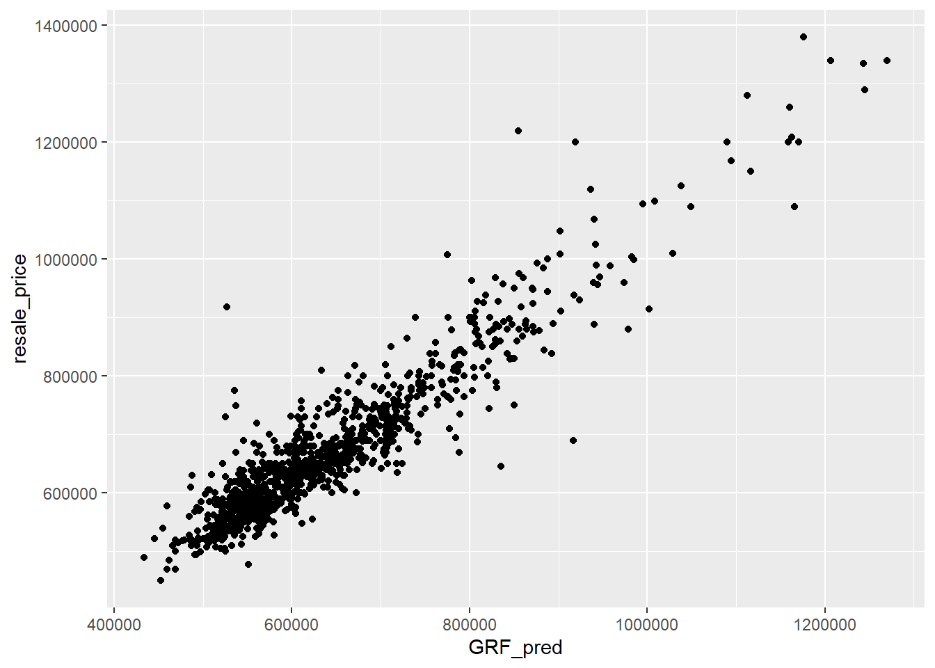
The above graph indicates a good fit of the GWR random forest model as points are distributed along the diagonal line.
9 Conclusion
Various methods and models - OLS, GWR and random forest - were used to derive a predictive model, revealing that the GWR model had performed better than the global regression model. The random forest model also performed well with test data as seen from section 8.4. The model was derived for 5 room HDB resale flats in Singapore based on the following independent variables:
Structural factors
Area of the unit
Floor level
Remaining lease
Locational factors
Proxomity to CBD
Proximity to eldercare
Proximity to hawker centres
Proximity to MRT
Proximity to park
Proximity to good primary school
Proximity to shopping mall
Proximity to supermarket
Number of kindergartens within 350m
Number of childcare centres within 350m
Number of bus stop within 350m
Number of primary schools within 1km