pacman::p_load(sf, tmap, tidyverse, sfdep)In-class Exercise 6: Spatial Weights and Applications using sfdep
1 Getting Started
2 Installing and loading R packages
3 Importing the data
3.1 Geospatial data
hunan <- st_read(dsn="data/geospatial",
                     layer="Hunan") %>% st_transform(crs=4480)
Reading layer `Hunan' from data source
`C:\annatrw\IS415\In-class_Ex\In-class_Ex06\data\geospatial'
using driver `ESRI Shapefile'
Simple feature collection with 88 features and 7 fields
Geometry type: POLYGON
Dimension: XY
Bounding box: xmin: 108.7831 ymin: 24.6342 xmax: 114.2544 ymax: 30.12812
Geodetic CRS: WGS 843.2 Aspatial data
pop2012 <- read_csv("data/aspatial/Hunan_2012.csv")head( list(pop2012), n=10)[[1]]
# A tibble: 88 × 29
County City avg_w…¹ depos…² FAI Gov_Rev Gov_Exp GDP GDPPC GIO
<chr> <chr> <dbl> <dbl> <dbl> <dbl> <dbl> <dbl> <dbl> <dbl>
1 Anhua Yiyang 30544 10967 6832. 457. 2703 13225 14567 9277.
2 Anren Chenzhou 28058 4599. 6386. 221. 1455. 4941. 12761 4189.
3 Anxiang Changde 31935 5517. 3541 244. 1780. 12482 23667 5109.
4 Baojing Hunan W… 30843 2250 1005. 193. 1379. 4088. 14563 3624.
5 Chaling Zhuzhou 31251 8241. 6508. 620. 1947 11585 20078 9158.
6 Changning Hengyang 28518 10860 7920 770. 2632. 19886 24418 37392
7 Changsha Changsha 54540 24332 33624 5350 7886. 88009 88656 51361
8 Chengbu Shaoyang 28597 2581. 1922. 161. 1192. 2570. 10132 1681.
9 Chenxi Huaihua 33580 4990 5818. 460. 1724. 7755. 17026 6644.
10 Cili Zhangji… 33099 8117. 4498. 500. 2306. 11378 18714 5843.
# … with 78 more rows, 19 more variables: Loan <dbl>, NIPCR <dbl>, Bed <dbl>,
# Emp <dbl>, EmpR <dbl>, EmpRT <dbl>, Pri_Stu <dbl>, Sec_Stu <dbl>,
# Household <dbl>, Household_R <dbl>, NOIP <dbl>, Pop_R <dbl>, RSCG <dbl>,
# Pop_T <dbl>, Agri <dbl>, Service <dbl>, Disp_Inc <dbl>, RORP <dbl>,
# ROREmp <dbl>, and abbreviated variable names ¹avg_wage, ²deposite4 Combining spatial and aspatial data
Both datasets have different columns, hence if we want to retain the geometry column from the geospatial data, left input file should be the one with geometry column; the right input file should be the aspatial data.
Note
Check if the unique identifier from both datasets are identical when performing any joins as R is case sensitive.
Note
columns selected are based on the output produced after the join, thereafter selecting columns 1 to 4, 7 and 15 which retains the GDP per capita from aspatial data.
hunan_join <- left_join(hunan, pop2012)%>%
  select(1:4, 7, 15)
5 Choropleth map of Hunan, GDP per capita
tmap_mode("plot")
tm_shape(hunan_join) +
  tm_fill('GDPPC',
          style= "quantile",
          palette = "Blues",
          title= "GDP per capita") +
  tm_layout(main.title = "Distribution of GDP per captia by district, Hunan province",
            main.title.position= "center",
            main.title.size = 1.2,
            legend.height=0.45,
            legend.width=0.35,
            frame=TRUE)+
  tm_borders(alpha=0.5)+
  tm_compass(type='8star', size =2) +
  tm_scale_bar()+
  tm_grid(alpha=0.2)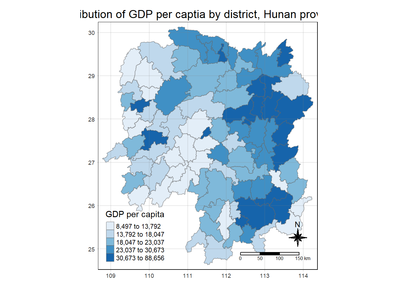
6 Contiguity neighbours method
Read the st-contiguity() method documentation <ahref=“https://sfdep.josiahparry.com/reference/st_contiguity.html”> here.
Note
This method is equivalent to the spdep package function poly2nb() used in Hands-On 6.
6.1 Queen method
Note
.before = 1 places the newly created field in the first column of hunan_join dataframe.
cn_queen <- hunan_join %>% mutate(nb= st_contiguity(geometry), .before=1)- the generated output cn_queen ’s nb column shows the nearest neighbours that are referenced by the index
- ie: the first data point Anxiang county has the following nearest neighbours: c(2,3,57,85) which refers to Hanshou, Jinshi, Li, Nan and Taoyuan.
6.2 Rook method
cn_rook <- hunan_join %>% mutate(nb= st_contiguity(geometry), queen=FALSE, .before=1)7 Contiguity weight matrix
7.1 Queen method
wm_q <- hunan_join %>%
  mutate(nb= st_contiguity(geometry),
         wt = st_weights(nb),
.before=1)- this code chunk allow the running of nearest neighbour using queen method and calculation of the weights
- generated output will include both the nearest neighbours and weights in the same dataframe
7.2 Rook method
wm_r <- hunan_join %>%
  mutate(nb= st_contiguity(geometry),
         queen= FALSE,
         wt = st_weights(nb),
         .before=1)