Show the code
pacman::p_load(sf, tidyverse,funModeling)Water is an important resource to mankind. Clean and accessible water is critical to human health. It provides a healthy environment, a sustainable economy, reduces poverty and ensures peace and security. Yet over 40% of the global population does not have access to sufficient clean water. By 2025, 1.8 billion people will be living in countries or regions with absolute water scarcity, according to UN-Water. The lack of water poses a major threat to several sectors, including food security. Agriculture uses about 70% of the world’s accessible freshwater.
Developing countries are most affected by water shortages and poor water quality. Up to 80% of illnesses in the developing world are linked to inadequate water and sanitation. Despite technological advancement, providing clean water to the rural community is still a major development issues in many countries globally, especially countries in the Africa continent.
To address the issue of providing clean and sustainable water supply to the rural community, a global Water Point Data Exchange (WPdx) project has been initiated. The main aim of this initiative is to collect water point related data from rural areas at the water point or small water scheme level and share the data via WPdx Data Repository, a cloud-based data library. What is so special of this project is that data are collected based on WPDx Data Standard.
The specific tasks of this take-home exercise are as follows:
pacman::p_load(sf, tidyverse,funModeling)geoNGA <- st_read("data/geospatial/", layer="geoBoundaries-NGA-ADM2") %>% st_transform(crs= 26392)Reading layer `geoBoundaries-NGA-ADM2' from data source
`C:\annatrw\IS415\In-class_Ex\In-class_Ex02\data\geospatial'
using driver `ESRI Shapefile'
Simple feature collection with 774 features and 6 fields
Geometry type: MULTIPOLYGON
Dimension: XY
Bounding box: xmin: 2.668534 ymin: 4.273007 xmax: 14.67882 ymax: 13.89442
Geodetic CRS: WGS 84NGA <- st_read("data/geospatial/",
layer = "nga_admbnda_adm2_osgof_20190417") %>%
st_transform(crs = 26392)Reading layer `nga_admbnda_adm2_osgof_20190417' from data source
`C:\annatrw\IS415\In-class_Ex\In-class_Ex02\data\geospatial'
using driver `ESRI Shapefile'
Simple feature collection with 774 features and 16 fields
Geometry type: MULTIPOLYGON
Dimension: XY
Bounding box: xmin: 2.668534 ymin: 4.273007 xmax: 14.67882 ymax: 13.89442
Geodetic CRS: WGS 84Waterpoint data from Humanitarian website
wp_nga <- read_csv("data/aspatial/WPdx.csv") %>%
filter(`#clean_country_name` == "Nigeria")Converts aspatial data into a simple feature object because aspatial data does not have geospatial information although latitude and londitude columns are present in the dataset. The function st_as_sfc() converts the selected column into a tibble data frame.
wp_nga$Geometry = st_as_sfc(wp_nga$`New Georeferenced Column`)
wp_nga
# A tibble: 95,008 × 71
row_id `#source` #lat_…¹ #lon_…² #repo…³ #stat…⁴ #wate…⁵ #wate…⁶ #wate…⁷
<dbl> <chr> <dbl> <dbl> <chr> <chr> <chr> <chr> <chr>
1 429068 GRID3 7.98 5.12 08/29/… Unknown <NA> <NA> Tapsta…
2 222071 Federal Minis… 6.96 3.60 08/16/… Yes Boreho… Well Mechan…
3 160612 WaterAid 6.49 7.93 12/04/… Yes Boreho… Well Hand P…
4 160669 WaterAid 6.73 7.65 12/04/… Yes Boreho… Well <NA>
5 160642 WaterAid 6.78 7.66 12/04/… Yes Boreho… Well Hand P…
6 160628 WaterAid 6.96 7.78 12/04/… Yes Boreho… Well Hand P…
7 160632 WaterAid 7.02 7.84 12/04/… Yes Boreho… Well Hand P…
8 642747 Living Water … 7.33 8.98 10/03/… Yes Boreho… Well Mechan…
9 642456 Living Water … 7.17 9.11 10/03/… Yes Boreho… Well Hand P…
10 641347 Living Water … 7.20 9.22 03/28/… Yes Boreho… Well Hand P…
# … with 94,998 more rows, 62 more variables: `#water_tech_category` <chr>,
# `#facility_type` <chr>, `#clean_country_name` <chr>, `#clean_adm1` <chr>,
# `#clean_adm2` <chr>, `#clean_adm3` <chr>, `#clean_adm4` <chr>,
# `#install_year` <dbl>, `#installer` <chr>, `#rehab_year` <lgl>,
# `#rehabilitator` <lgl>, `#management_clean` <chr>, `#status_clean` <chr>,
# `#pay` <chr>, `#fecal_coliform_presence` <chr>,
# `#fecal_coliform_value` <dbl>, `#subjective_quality` <chr>, …wp_sf <- st_sf(wp_nga, crs=4326)
wp_sf <- wp_sf %>% st_transform(crs=26392)Removing redundant fields using dplyr select()
NGA <- NGA %>% select (c(3:4,8:9))Checking for duplicate name using Base R duplicated()
NGA$ADM2_EN[duplicated(NGA$ADM2_EN)==TRUE][1] "Bassa" "Ifelodun" "Irepodun" "Nasarawa" "Obi" "Surulere"The above code shows the duplicated fields with the same name from different states (ADM1_PCODE).
To fix the duplicated values, replace the duplicated rows with
NGA$ADM2_EN[94] <- "Bassa, Kogi"
NGA$ADM2_EN[95] <- "Bassa, Plateau"
NGA$ADM2_EN[304] <- "Ifelodun, Kwara"
NGA$ADM2_EN[305] <- "Ifelodun, Osun"
NGA$ADM2_EN[355] <- "Irepodun, Kwara"
NGA$ADM2_EN[356] <- "Irepodun, Osun"
NGA$ADM2_EN[519] <- "Nasarawa, Kano"
NGA$ADM2_EN[520] <- "Nasarawa, Nasarawa"
NGA$ADM2_EN[546] <- "Obi, Benue"
NGA$ADM2_EN[547] <- "Obi, Nasarawa"
NGA$ADM2_EN[693] <- "Surulere, Lagos"
NGA$ADM2_EN[694] <- "Surulere, Oyo"freq(data = wp_sf,
input = '#status_clean')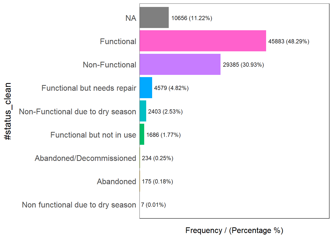
                     #status_clean frequency percentage cumulative_perc
1                       Functional     45883      48.29           48.29
2                   Non-Functional     29385      30.93           79.22
3                             <NA>     10656      11.22           90.44
4      Functional but needs repair      4579       4.82           95.26
5 Non-Functional due to dry season      2403       2.53           97.79
6        Functional but not in use      1686       1.77           99.56
7         Abandoned/Decommissioned       234       0.25           99.81
8                        Abandoned       175       0.18           99.99
9 Non functional due to dry season         7       0.01          100.00
rename() is used to rename the column from #status_clean to status_clean (removing the hash icon)
select() is used to include status_clean in the outputs of sf data frame
mutate() and replace_na() replaces the NA values in status_clean field into ‘unknown’
wp_sf_nga <- wp_sf %>%
  rename(status_clean = '#status_clean') %>%
  select(status_clean) %>%
mutate(status_clean = replace_na(status_clean, "unknown"))Functional water point data
wp_functional <- wp_sf_nga %>%
  filter(status_clean %in%
  c("Functional", "Functional but not in use", "Functional but needs repair"))
Non-functional water point data
wp_nonfunctional <- wp_sf_nga %>%
  filter(status_clean %in%
  c("Abandoned/Decommissioned", "Abandoned", "Non-Functional due to dry season", "Non-Functional","Non functional due to dry season"))
wp_unkown <- wp_sf_nga %>%
filter(status_clean == "unknown")Finding water points that fall within each LGA length() used to calculate number of water points
NGA_wp <- NGA %>%
  mutate(`total_wp` = lengths(st_intersects(NGA, wp_sf_nga))) %>%
  mutate(`wp_functional` = lengths(st_intersects(NGA, wp_functional))) %>%
  mutate(`wp_nonfunctional` = lengths(st_intersects(NGA, wp_nonfunctional))) %>%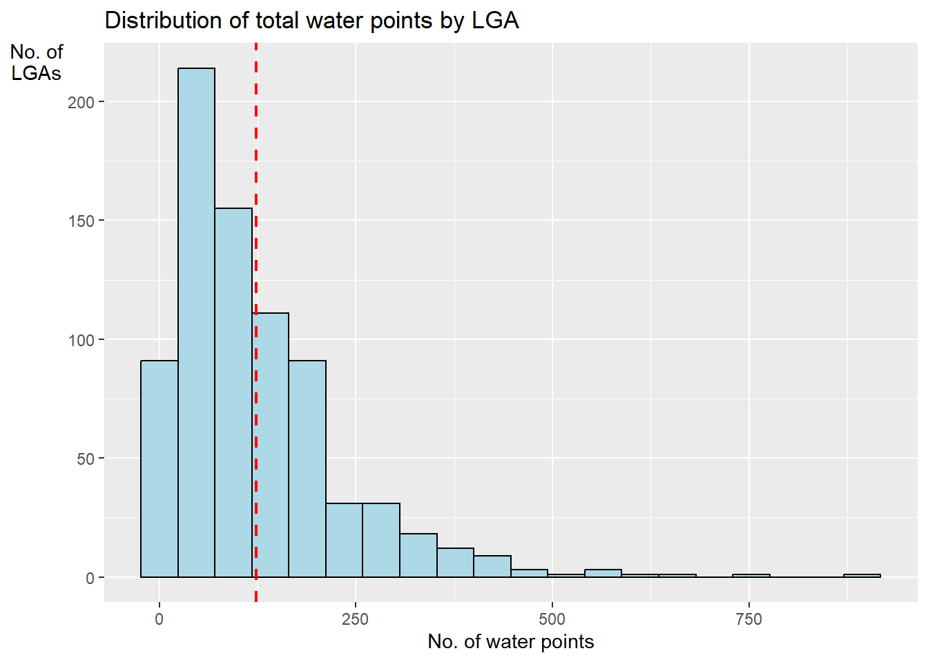
mutate(`wp_unknown` = lengths(st_intersects(NGA, wp_unkown)))write_rds(NGA_wp, "data/rds/NGA_wp.rds")Using ggplot2 to visualise distribution of water points.
ggplot(data = NGA_wp, aes(x=total_wp)) + geom_histogram(bins=20, color="black", fill="light blue") +
  geom_vline(aes(xintercept=mean(total_wp, na.rm=T)), color="red", linetype="dashed", size = 0.8 ) +
  ggtitle("Distribution of total water points by LGA") +
  xlab("No. of water points") +
  ylab ("No. of\nLGAs") +
  theme(axis.title.y=element_text(angle=0))